chapter3_1

데이터 준비

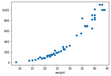
import numpy as np

perch_length = np.array(
    [8.4, 13.7, 15.0, 16.2, 17.4, 18.0, 18.7, 19.0, 19.6, 20.0, 
     21.0, 21.0, 21.0, 21.3, 22.0, 22.0, 22.0, 22.0, 22.0, 22.5, 
     22.5, 22.7, 23.0, 23.5, 24.0, 24.0, 24.6, 25.0, 25.6, 26.5, 
     27.3, 27.5, 27.5, 27.5, 28.0, 28.7, 30.0, 32.8, 34.5, 35.0, 
     36.5, 36.0, 37.0, 37.0, 39.0, 39.0, 39.0, 40.0, 40.0, 40.0, 
     40.0, 42.0, 43.0, 43.0, 43.5, 44.0]
     )
perch_weight = np.array(
    [5.9, 32.0, 40.0, 51.5, 70.0, 100.0, 78.0, 80.0, 85.0, 85.0, 
     110.0, 115.0, 125.0, 130.0, 120.0, 120.0, 130.0, 135.0, 110.0, 
     130.0, 150.0, 145.0, 150.0, 170.0, 225.0, 145.0, 188.0, 180.0, 
     197.0, 218.0, 300.0, 260.0, 265.0, 250.0, 250.0, 300.0, 320.0, 
     514.0, 556.0, 840.0, 685.0, 700.0, 700.0, 690.0, 900.0, 650.0, 
     820.0, 850.0, 900.0, 1015.0, 820.0, 1100.0, 1000.0, 1100.0, 
     1000.0, 1000.0]
     )

k-최근점 이웃 회귀(Regression)

• 중요도 : 하 (그냥 넘어가세요!)
  • 실무에서 잘 안쓰이고, 시간은 한정되어 있기 때문

시각화

• 다음과 같이 fig, ax를 이용해 객체 지향으로 작성하라

import matplotlib.pyplot as plt

# 객체 지향으로 변경
fig, ax = plt.subplots()
ax.scatter(perch_length, perch_weight)
ax.set_xlabel("length")
ax.set_xlabel("weight")

plt.show()

훈련데이터 테스트데이터셋 분리

• 외워야 할 정도로 중요하다.

from sklearn.model_selection import train_test_split
train_input, test_input, train_target, test_target = train_test_split(  # 자체적으로 셔플이 된다.
    perch_length, perch_weight, random_state = 42
)

train_input.shape, test_input.shape, train_target.shape, test_target.shape

((42,), (14,), (42,), (14,))

• reshape() 사용하여 2차원 배열로 바꿈

train_input = train_input.reshape(-1, 1)
test_input = test_input.reshape(-1, 1)

print(train_input.shape, test_input.shape)

(42, 1) (14, 1)

결정계수

• 모델이 얼마만큼 정확하냐?

from sklearn.neighbors import KNeighborsRegressor

# knn 클래스 불러오기
knr = KNeighborsRegressor()

# 모형학습
knr.fit(train_input, train_target)

# 테스트 점수 확인하자
knr.score(test_input, test_target)

0.992809406101064

MAE

• 타깃과 예측의 절댓값 오차를 평균하여 반환

from sklearn.metrics import mean_absolute_error

# 예측 데이터 만들기
test_prediction = knr.predict(test_input)
test_prediction

array([  60. ,   79.6,  248. ,  122. ,  136. ,  847. ,  311.4,  183.4,
        847. ,  113. , 1010. ,   60. ,  248. ,  248. ])

• mae를 구한다.
• mae = mean_absolute_error
  • 평균적 오차를 구하는 것이다.

mae = mean_absolute_error(test_target, test_prediction)
print(mae)

• 평균적으로 19g정도 다르다.

과대적합 vs 과소적합

• 공통점은 머신러닝 모형이 실제 테스트 시 잘 예측을 못함!
• 과대적합 : 훈련데이터에는 예측 잘함 / 테스트 데이터에서는 예측을 잘 못함
  • 처리하기 곤란
• 과소적합 : 훈련데이터에서는 예측을 못하고, 테스트데이터에서는 예측을 잘 함 or 둘다 예측을 잘 못함.
  • 데이터의 양이 적거나, 모델을 너무 간단하게 만듬!

# 훈련 데이터 점수 확인하자.
knr.score(train_input, train_target)

0.9698823289099254

• 0.97 정도 나옴

# Defult 5를 3으로 변경
# 머신러닝 모형을 살짝 변경
knr.n_neighbors = 3

# 모델을 다시 훈련
knr.fit(train_input, train_target)
print(knr.score(train_input, train_target))

0.9804899950518966

• 훈련데이터로 검증 0.98

print(knr.score(test_input, test_target))

0.9746459963987609

• mae 구하기
  • 평균적 오차 구하기

test_prediction = knr.predict(test_input)
mae = mean_absolute_error(test_target, test_prediction)
print(mae)

35.42380952380951

• 평균적으로 35.4g 다름

결론

• k 그룹을 5로 했을 때, R2 점수는 0.98, MAE는 19 였음

• k 그룹을 3로 했을 때, R2 점수는 0.97, MAE는 35 였음

• k 그룹을 7로 했을 때, R2 점수는 0.97, MAE는 32 였음

• Reference : 혼자 공부하는 머신러닝 + 딥러닝