1
2
3
4
5
6
7
8
9
10
11
12
13
14
15
16
17
18
19
20
21
22
23
24
25
26
27
28
29
30
31
32
33
34
35
36
37
38
39
40
41
42
43
44
45
46
47
48
49
50
51
52
53
54
55
56
57
58
59
60
61
62
63
64
65
66
67
68
69
70
71
72
73
74
75
76
77
78
79
80
81
82
83
84
85
86
87
88
89
90
91
92
93
94
95
96
97
98
99
100
101
102
103
104
105
106
107
108
109
110
111
112
113
114
115
116
117
118
| import numpy as np
perch_length = np.array(
[8.4, 13.7, 15.0, 16.2, 17.4, 18.0, 18.7, 19.0, 19.6, 20.0,
21.0, 21.0, 21.0, 21.3, 22.0, 22.0, 22.0, 22.0, 22.0, 22.5,
22.5, 22.7, 23.0, 23.5, 24.0, 24.0, 24.6, 25.0, 25.6, 26.5,
27.3, 27.5, 27.5, 27.5, 28.0, 28.7, 30.0, 32.8, 34.5, 35.0,
36.5, 36.0, 37.0, 37.0, 39.0, 39.0, 39.0, 40.0, 40.0, 40.0,
40.0, 42.0, 43.0, 43.0, 43.5, 44.0]
)
perch_weight = np.array(
[5.9, 32.0, 40.0, 51.5, 70.0, 100.0, 78.0, 80.0, 85.0, 85.0,
110.0, 115.0, 125.0, 130.0, 120.0, 120.0, 130.0, 135.0, 110.0,
130.0, 150.0, 145.0, 150.0, 170.0, 225.0, 145.0, 188.0, 180.0,
197.0, 218.0, 300.0, 260.0, 265.0, 250.0, 250.0, 300.0, 320.0,
514.0, 556.0, 840.0, 685.0, 700.0, 700.0, 690.0, 900.0, 650.0,
820.0, 850.0, 900.0, 1015.0, 820.0, 1100.0, 1000.0, 1100.0,
1000.0, 1000.0]
)
from sklearn.model_selection import train_test_split
train_input, test_input, train_target, test_target = train_test_split(
perch_length, perch_weight, random_state=42)
train_input = train_input.reshape(-1, 1)
test_input = test_input.reshape(-1, 1)
from sklearn.neighbors import KNeighborsRegressor
knr = KNeighborsRegressor(n_neighbors=3)
knr.fit(train_input, train_target)
print(knr.predict([[50]]))
import matplotlib.pyplot as plt
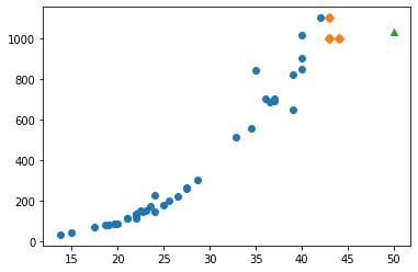
distances, indexes = knr.kneighbors([[50]])
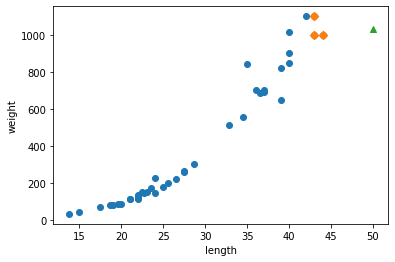
plt.scatter(train_input, train_target)
plt.scatter(train_input[indexes], train_target[indexes], marker='D')
plt.scatter(50, 1033, marker='^')
plt.xlabel('length')
plt.ylabel('weight')
plt.show()
print(np.mean(train_target[indexes]))
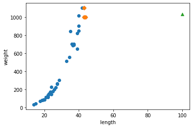
print(knr.predict([[100]]))
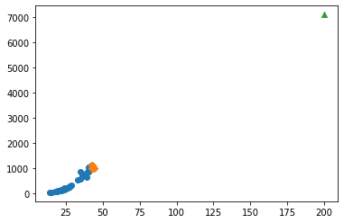
distances, indexes = knr.kneighbors([[100]])
plt.scatter(train_input, train_target)
plt.scatter(train_input[indexes], train_target[indexes], marker='D')
plt.scatter(100, 1033, marker='^')
plt.xlabel('length')
plt.ylabel('weight')
plt.show()
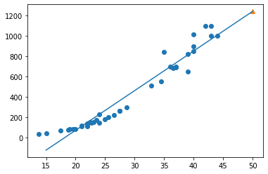
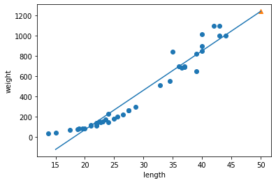
from sklearn.linear_model import LinearRegression
lr = LinearRegression()
lr.fit(train_input, train_target)
print(lr.predict([[50]]))
print(lr.coef_, lr.intercept_)
plt.scatter(train_input, train_target)
plt.plot([15, 50], [15*lr.coef_+lr.intercept_, 50*lr.coef_+lr.intercept_])
plt.scatter(50, 1241.8, marker='^')
plt.xlabel('length')
plt.ylabel('weight')
plt.show()
print(lr.score(train_input, train_target))
print(lr.score(test_input, test_target))
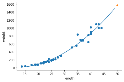
train_poly = np.column_stack((train_input ** 2, train_input))
test_poly = np.column_stack((test_input ** 2, test_input))

print(train_poly.shape, test_poly.shape)
lr = LinearRegression()
lr.fit(train_poly, train_target)
print(lr.predict([[50**2, 50]]))
print(lr.coef_, lr.intercept_)
point = np.arange(15, 50)
plt.scatter(train_input, train_target)
plt.plot(point, 1.01*point**2 - 21.6*point + 116.05)
plt.scatter([50], [1574], marker='^')
plt.xlabel('length')
plt.ylabel('weight')
plt.show()
print(lr.score(train_poly, train_target))
print(lr.score(test_poly, test_target))
|