• Spark로 머신러닝을 사용해 본다.
• 실용성과 별개로 경험삼아 작성해보는 코드이다.
• 머신러닝(ML)은 Scikit-Learn을 중점적으로 공부해야 한다.
• 딥러닝(DL)은 Tensorflow, Pytorch에 포커스를 맞춰야 한다.

사전준비

• git bash로 VSCord에 들어가 터밀널을 연다.

바탕화면 우클릭 : git bash here

→ cd pyspk_project

→ code .

→ git bash 터미널

pyspark_ml 실습(1)

• 가상환경 진입하고 폴더, 파일 생성

→ source venv/Scripts/activate

→ 폴더 생성 : chapter03_ml

→ cd chapter03_ml

• 슬랙에서 data.zip 을 다운로드
• 압축을 풀고 chapter03_ml 폴더에 복사하여 옮긴다.

→ 파일 생성 : step01_regression.py

→ 코드 작성

1
2
3
4
5
6
7
8
9
10
11
12
13
14
15
16
17
18
19
20
21
22
23
24
25
26
27
28
29
30
31
32
33
34
35
36
37
38
39
40
41
42
43
44
45
46
47
48

from pyspark.ml.regression import DecisionTreeRegressor
from pyspark.sql import SparkSession
from pyspark.ml.feature import VectorAssembler

# 세션 할당
spark = SparkSession.builder.appName("DecisionTree").getOrCreate()

# 데이터 불러오기
# StructType 이 과정 생략
data = spark.read.option("header", "true").option("inferSchema", "true").csv("data/realestate.csv")

# 데이터 프레임을 행렬로 변환
assembler = VectorAssembler().setInputCols(['HouseAge', 'DistanceToMRT', 'NumberConvenienceStores']).setOutputCol("features")

# 타겟데이터 설정
df = assembler.transform(data).select("PriceofUnitArea", "features")

# 데이터 분리
trainTest = df.randomSplit([0.5, 0.5])
trainingDF = trainTest[0]
testDF = trainTest[1]

# Decision Tree 클래스 정의
dtr = DecisionTreeRegressor().setFeaturesCol("features").setLabelCol("PriceofUnitArea")

# 모델 학습
model = dtr.fit(trainingDF)
print(model)

# 모델 예측
fullPredictions = model.transform(testDF).cache()

# 예측값과 Label을 분리
predictions = fullPredictions.select("prediction").rdd.map(lambda x: x[0])

# 실제데이터
labels = fullPredictions.select("PriceofUnitArea").rdd.map(lambda x: x[0])

# zip
preds_label = predictions.zip(labels).collect()

for prediction in preds_label:
    print(prediction)

# print(data.show())

# 세션 종료
spark.stop()

→ 저장 후 실행

→ python step01_regression.py

→ 다음과 같이 출력된다.

pyspark_ml 실습(2)

→ 파일 생성 : step02_logistic_regression.py

→ 코드 작성

1
2
3
4
5
6
7
8
9
10
11
12
13
14
15
16
17
18
19
20

# 세션 할당
from pyspark.sql import SparkSession
from pyspark.ml.classification import LogisticRegression # 기억

spark = SparkSession.builder.appName("AppName").getOrCreate()

# 데이터 불러오기
training = spark.read.format("libsvm").load("data/mllib/sample_libsvm_data.txt")
print("hello")

# 모델 만들기
# Scikit-Learn 문법과 비슷
mlr = LogisticRegression() # 기억
mlr_model = mlr.fit(training) # 기억

# 로지스틱 회귀, 선형 모델.. 기울기와 상수
print("Coefficients: " + str(mlr_model.coefficients))
print("Intercept: " + str(mlr_model.intercept))

spark.stop()

→ 저장 후 실행

→ python step02_logistic_regression.py

pyspark_ml 실습(3)

• pyspark_pipeline

→ 파일 생성 : step03_pipeline.py

→ 코드 작성

1
2
3
4
5
6
7
8
9
10
11
12
13
14
15
16
17
18
19
20
21
22
23
24
25
26
27
28
29
30
31
32
33
34
35
36
37
38
39
40
41
42
43
44
45
46
47
48
49
50
51
52
53
54
55
56
57
58

from tokenize import Token
from pyspark.ml import Pipeline
from pyspark.ml.classification import LogisticRegression
from pyspark.ml.feature import HashingTF, Tokenizer

from pyspark.sql import SparkSession

# 세션 할당
spark = SparkSession.builder.appName("MLPipeline").getOrCreate()

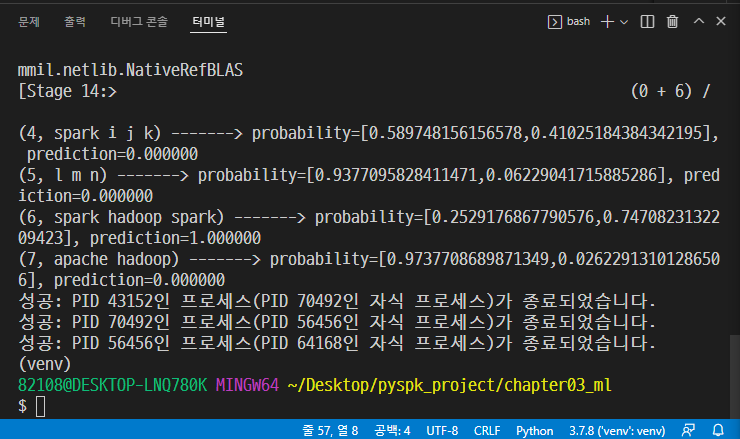
# 가상의 데이터 만들기
training = spark.createDataFrame([
    (0, "a b c d e spark", 1.0),
    (1, "b d", 0.0),
    (2, "spark f g h", 1.0),
    (3, "hadoop mapreduce", 0.0)
], ["id", "text", "label"])

# Feature Engineering
# 요리 작업

# 요리준비 1단계 : 텍스트를 단어로 분리
tokenizer = Tokenizer(inputCol='text', outputCol='words')

# 요리준비 2단계 : 변환된 텍스트를 숫자로 변환
hashingTF = HashingTF(inputCol=tokenizer.getOutputCol(), outputCol="features")

# 요리준비 3단계 : 모델을 가져옴
lr = LogisticRegression(maxIter=5, regParam=0.01)

# 요리 시작
pipeline = Pipeline(stages=[tokenizer, hashingTF, lr])

# 메인재료 투하
model = pipeline.fit(training)

# Prepare test documents, which are unlabeled (id, text) tuples.
test = spark.createDataFrame([
    (4, "spark i j k"),
    (5, "l m n"),
    (6, "spark hadoop spark"),
    (7, "apache hadoop")
], ["id", "text"])

# 예측
prediction = model.transform(test)
selected = prediction.select("id", "text", "probability", "prediction")
for row in selected.collect():
    row_id, text, prob, prediction = row # 튜플
    print(
        # 문자열 포맷팅
        "(%d, %s) -------> probability=%s, prediction=%f" % (row_id, text, str(prob), prediction)
    )

# training.show()

# 세션 종료
spark.stop()

→ 저장 후 실행

→ python step03_pipeline.py

pyspark_ml 실습(3)

→ 파일 생성 : step03_randomforest.py

→ 코드 작성

1
2
3
4
5
6
7
8
9
10
11
12
13
14
15
16
17
18
19
20
21
22
23
24
25
26
27
28
29
30
31
32
33
34
35
36
37
38
39
40
41
42
43
44
45
46
47
48
49
50
51
52
53
54
55
56

from cProfile import label
from pyspark.sql import SparkSession

# 머신러닝 라이브러리
from pyspark.ml import Pipeline
from pyspark.ml.classification import RandomForestClassifier
from pyspark.ml.feature import IndexToString, StringIndexer, VectorIndexer
from pyspark.ml.evaluation import MulticlassClassificationEvaluator

# 데이터 불러오기
spark = SparkSession.builder.appName("RandomForest").getOrCreate()

data = spark.read.format("libsvm").load("data/mllib/sample_libsvm_data.txt")
print(type(data))

# Feature Engineering
# label column
labelIndexer = StringIndexer(inputCol='label', outputCol='indexedLabel').fit(data)

# 범주형 데이터 체크, 인덱스화
featureIndexer = VectorIndexer(inputCol='features',
                               outputCol='IndexedFeatures', maxCategories=4).fit(data)

# 데이터 분리
(trainingData, testData) = data.randomSplit([0.7, 0.3])

# 모델
rf = RandomForestClassifier(labelCol='indexedLabel', # 종속변수
                            featuresCol='IndexedFeatures', # 독립변수
                            numTrees=10)

# outputCol='indexedLabel' --> original label로 변환
labelConvereter = IndexToString(inputCol='prediction',
                                outputCol='predictedLabel', labels=labelIndexer.labels)

# 파이프라인 구축
pipeline = Pipeline(stages=[labelIndexer, featureIndexer, rf, labelConvereter])

# 모델 학습
model = pipeline.fit(trainingData)

# 모델 예측
predictions = model.transform(testData)

# 행에 표시할 것 추출
predictions.select("predictedLabel", 'label', 'features').show(5)

# 모형 평가
evaluator = MulticlassClassificationEvaluator(
    labelCol="indexedLabel", predictionCol="prediction", metricName="accuracy"
)

accuracy = evaluator.evaluate(predictions)
print("Test Error = %f " % (1.0 - accuracy))

spark.stop()

→ 저장 후 실행

→ python step04_randomforest.py

팁

venv 생성되어 있는 경로로 이동

→ pip install jupyterlab

→ jupyter lab

→ 주피터랩에서 블로그에 올릴 자료 작성 가능.

• Reference : https://spark.apache.org/docs/latest/api/python/reference/api/pyspark.sql.types.StructType.html

사전준비

• git bash로 VSCord에 들어가 터밀널을 연다.

바탕화면 우클릭 : git bash here

→ cd pyspk_project

→ code .

→ git bash 터미널

pyspark 실습(1)

• 가상환경 진입하고 폴더, 파일 생성

→ source venv/Scripts/activate

→ 폴더 생성 : chapter02_get_cleansing

• 슬랙에서 data.zip 을 다운로드
• 압축을 풀고 chapter02_get_cleansing 파일에 복사하여 옮긴다.

→ 파일 생성 : pipeline.py

• 코드를 작성해본다.

→ 코드 작성

from pyspark.sql import SparkSession

from pyspark.sql.functions import *

print("Hello!")

→ 저장

→ 경로 이동 : cd chapter02_get_cleansing

→ 실행 : python pipeline.py

• 이어서 코드작성

→ pipeline.py를 다음과 같이 작성

1
2
3
4
5
6
7
8
9
10
11
12
13
14
15
16
17
18
19
20
21
22
23
24
25
26
27
28

from pyspark.sql import SparkSession
from pyspark.sql.functions import *
from pyspark.sql import functions as F

# print("Hello!!")

# 스파크 세션을 생성
spark = SparkSession.builder.master("local[1]").\
    appName("quickpipeline").getOrCreate()

# 데이터 불러오기
df = spark.read.csv("data\AA_DFW_2015_Departures_Short.csv.gz"
                    , header = True)

print("file loaded")

print(df.show())

# remove duration = 0
df = df.filter(df[3] > 0)

# ADD ID column
df = df.withColumn('id', F.monotonically_increasing_id())
df.show()

df.write.csv("data/output.csv", mode = "overwrite")

spark.stop()

→ 저장 후 실행

→ python pipeline.py

→ output.csv 가 생성되면 성공이다.

pyspark 실습(2)

• 온도를 측정하는 코드를 작성해본다.
• 슬랙에서 다운로드
  • 1800.csv, book.txt, customer-orders.csv, fakefriends.csv
• chapter02_get_cleansing/data 파일에 복사하여 옮긴다.

파일 생성 : min_temp.py

→ 코드 작성

from pyspark import SparkConf, SparkContext

conf = SparkConf().setMaster('local').setAppName('MinTemperatures')

sc = SparkContext(conf = conf)

print("Hello")

→ 저장 후 실행

→ python min_temp.py

• 이어서 코드작성

→ min_temp.py를 다음과 같이 작성

from pyspark import SparkConf, SparkContext

conf = SparkConf().setMaster(‘local’).setAppName(‘MinTemperatures’)

sc = SparkContext(conf = conf)

print(“Begins…”)

def parseLine(line):

fileds = line.split(‘,’) # 문자열을 split

stationID = fileds[0]

entryType = fileds[2]

temperature = float(fileds[3]) * 0.1 * (9.0 / 5.0) + 32.0

return (stationID, entryType, temperature)

lines = sc.textFile(‘data/1800.csv’)

#print(lines)

parseLines = lines.map(parseLine)

#print(parseLine)

minTemps = parseLine.filter(lambda x : “TMIN” in x[1])

stationTemps = minTemps.map(lambda x: (x[0], x[2]))

minTemps = stationTemps.map(lambda x, y: min(x,y))

results = minTemps.collect()

print(results)

→ 저장 후 실행

→ python min_temp.py

pyspark 실습(3)

• 나이를 출력하는 코드를 작성해보자

파일 생성 : friends-by-age.py

→ 코드 작성

1
2
3
4
5
6
7
8
9
10
11
12
13
14
15
16
17
18

from pyspark import SparkConf, SparkContext

conf = SparkConf().setMaster("local").setAppName("FriendsByAge")
sc = SparkContext(conf = conf)

def parseLine(line):
    fields = line.split(',')
    age = int(fields[2])
    numFriends = int(fields[3])
    return (age, numFriends)

lines = sc.textFile("logs/fakefriends.csv")
rdd = lines.map(parseLine)
totalsByAge = rdd.mapValues(lambda x: (x, 1)).reduceByKey(lambda x, y: (x[0] + y[0], x[1] + y[1]))
averagesByAge = totalsByAge.mapValues(lambda x: x[0] / x[1])
results = averagesByAge.collect()
for result in results:
    print(result)

→ 저장 후 실행

→ python friends-by-age.py

pyspark 실습(4)

파일 생성 : totalspent.py

→ 코드 작성

1
2
3
4
5
6
7
8
9
10
11
12
13
14
15
16
17
18
19
20
21
22
23
24
25
26
27
28
29
30
31

# 라이브러리 불러오기
from pyspark import SparkConf, SparkContext

# 사용자 정의 함수
def extractCusPrice(line):
    fields = line.split(",")
    return (int(fields[0]), float(fields[2]))

# main 함수
def main():

    # 스파크 설정
    conf = SparkConf().setMaster("local").setAppName('SpentbyCustomer')
    sc = SparkContext(conf = conf)

    # 데이터 불러오기
    input = sc.textFile("data/customer-orders.csv")
    # print("is data?")
    mappedInput = input.map(extractCusPrice)
    totalByCustomer = mappedInput.reduceByKey(lambda x, y : x + y)
		# 정렬
    filpped = totalByCustomer.map(lambda x: (x[1], x[0]))
    totalByCustomerStored = filpped.sortByKey()

    results = totalByCustomer.collect()
    for result in results:
        print(result)

# 실행 코드
if __name__ == "__main__":
    main()

→ 저장 후 실행

→ python totalspent.py

• Reference : https://spark.apache.org/docs/latest/api/python/reference/api/pyspark.sql.types.StructType.html

사전준비

• git bash로 VSCord에 들어가 터미널을 연다.

바탕화면 우클릭 : git bash here

→ cd pyspk_project

→ code .

→ git bash 터미널

pyspark 실습(1)

• 가상환경 진입하고 파일 생성

→ source venv/Scripts/activate

→ chapter01_get_starged 폴더에서 파일 생성

→ 파일 생성 : step04_structype.py

키워드 : Struct Type

구글링 : Spark Struct Type, Spark Struct

참고 링크 :

https://spark.apache.org/docs/latest/api/python/reference/api/pyspark.sql.types.StructType.html

→ 코드 작성

1
2
3
4
5
6
7
8
9
10
11
12
13
14
15
16
17
18
19
20
21
22
23
24
25
26
27
28
29
30
31
32

from struct import Struct
from pyspark.sql import SparkSession
from pyspark.sql import functions as func 
from pyspark.sql.types import StructType, StructField, IntegerType, LongType

# 세션 할당 (필수)
# spark = SparkSession.builder.appName("")
spark = SparkSession.builder.appName("PopularMovies").getOrCreate()

# 스키마 작성 (u.logs 데이터)
schema = StructType(
    [
        StructField("userID", IntegerType(), True),
        StructField("movieID", IntegerType(), True),
        StructField("rating", IntegerType(), True),
        StructField("timestamp", LongType(), True)
    ]
) 

print("Schema is done")

# 데이터 불러오기
movies_df = spark.read.option("sep", "\t").schema(schema).csv("ml-100k/u.logs")

# 내림차순으로 인기있는 영화 정렬
# movieID 그룹바이. count() orderby
toMovieIds = movies_df.groupBy("movieID").count().orderBy(func.desc('count'))

print(movies_df.show(10))

# 세션 종료
spark.stop()

→ 경로 이동 : cd chapter01_get_started

→ 저장 후 실행

→ python step04_structype.py

→ 다음 테이블이 출력되어야 한다.

pyspark 실습(2)

→ chapter01_get_starged 폴더에서 파일 생성

→ 파일 생성 : step05_advancestructype.py

→ 코드 작성

1
2
3
4
5
6
7
8
9
10
11
12
13
14
15
16
17
18
19
20
21
22
23
24
25
26
27
28
29
30
31
32
33
34
35
36
37
38
39
40
41
42
43
44
45
46
47
48
49
50
51
52
53
54
55
56
57
58

from pyspark.sql import SparkSession
from pyspark.sql import functions as func
from pyspark.sql.types import StructType, StructField, IntegerType, LongType
import codecs

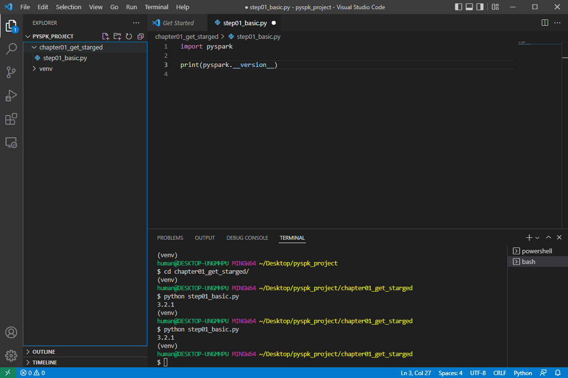
print("Hello")

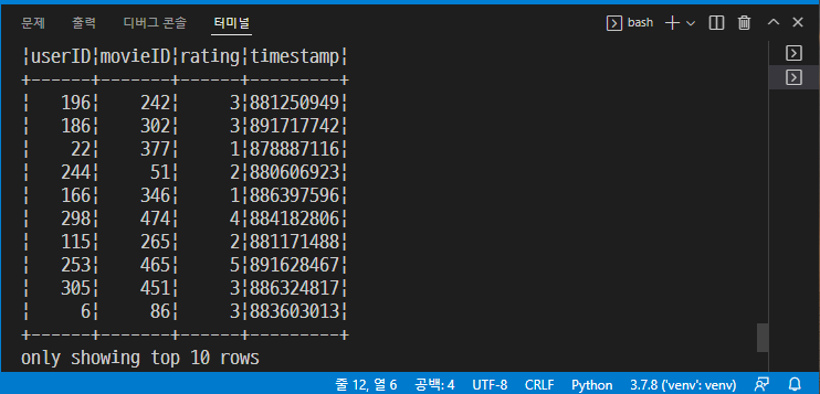
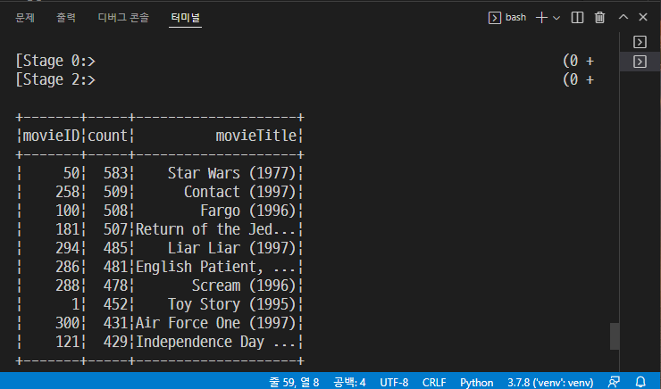
def loadMovieNames():
    movieNames = {}
    with codecs.open("ml-100k/u.ITEM", "r", encoding="ISO-8859-1", errors="ignore") as f:
        for line in f:
            fields = line.split("|")
            movieNames[int(fields[0])] = fields[1]
    return movieNames

# 세션 할당
spark = SparkSession.builder.appName("PopularMovies").getOrCreate()

# 파이썬 딕셔너리 객체를 Spark 객체로 변환
nameDict = spark.sparkContext.broadcast(loadMovieNames())

# 스키마 작성 (u.logs 데이터)
schema = StructType(
    [
        StructField("userID", IntegerType(), True)
        , StructField("movieID", IntegerType(), True)
        , StructField("rating", IntegerType(), True)
        , StructField("timestamp", LongType(), True)
    ]
)

print("Schema is done")

# 데이터 불러오기
movies_df = spark.read.option("sep", "\t").schema(schema).csv("ml-100k/u.logs")

# 내림차순으로 인기있는 영화 정렬
# movieID 그룹바이. count() orderby
topMovieIds = movies_df.groupBy("movieID").count()

# 딕셔너리
# key-value
# 키 값을 알면 value 자동으로 가져옴 (movieTitle)
def lookupName(movieID):
    return nameDict.value[movieID]

lookupNameUDF = func.udf(lookupName)

# MovieTitle 기존 topMovieIds 데이터에 추가
# 컬럼을 추가
moviesWithNames = topMovieIds.withColumn("movieTitle", lookupNameUDF(func.col("movieID")))

final_df = moviesWithNames.orderBy(func.desc("count"))

print(final_df.show(10))

# 세션 종료
spark.stop()

→ 저장 후 실행

→ python step05_advancestructype.py

→ 다음과 같이 출력된다.

• Reference : https://spark.apache.org/docs/latest/api/python/reference/api/pyspark.sql.types.StructType.html

사전준비

• spark on windows 참고하여 세팅
• 스파크를 설치한다.
• 만약, 파이썬이 처음이라면 **Anaconda**를 설치한다.

pyspark 설치

• git bash를 이용해 폴더를 생성하고 터미널을 연다.

바탕화면 우클릭 : git bash here

→ mkdir pyspk_project

→ cd pyspk_project

→ code .

→ git bash 터미널

• 가상환경 생성 후 pyspark 설치

→ virtualenv venv

→ source venv/Scripts/activate

→ pip install pyspark

pyspark 실습_1

• 폴더 파일 생성

→ 폴더 생성 : chapter01_get_started

→ 파일 생성 : step01_basic.py

→ 코드 작성

import pyspark

print(pyspark.__version__)

→ 저장

→ 경로 이동 : cd chapter01_get_started

→ 실행 : python step01_basic.py

• 이어서 코드작성

→ step01_basic.py를 다음과 같이 작성

1
2
3
4
5
6
7
8
9
10
11
12

# -*- coding: utf-8 -*-

import pyspark
print(pyspark.__version__)

from pyspark.sql import SparkSession

# 스파크 세션 초기화
spark = SparkSession.builder.master('local[1]').appName('SampleTutorial').getOrCreate()
rdd = spark.sparkContext.parallelize([1, 2, 3, 4, 5])

print("rdd Count:", rdd.count())

→ 저장 후 실행

→ 주소창에 입력 : http://localhost:4040/

→ 다음 화면이 출력된다.

• 교재 278p

pyspark 실습_2

• 슬랙에서 dataset.zip 을 다운로드
• 압축을 풀고 chapter01_get_started 파일에 복사하여 옮긴다.

• VSCord에서 작업

→ 파일 생성 : step02_ratings.py

→ 코드 작성

1
2
3
4
5
6
7
8
9
10
11
12
13
14
15
16
17
18
19
20
21
22
23
24
25
26
27
28

# SparkContext
# RDD

from pyspark import SparkConf, SparkContext
import collections

print("Hello")

def main():
    # MasterNode = local
    # MapReduce

    conf = SparkConf().setMaster('local').setAppName('RatingsHistogram')
    sc = SparkContext(conf = conf)

    lines = sc.textFile("ml-100k/u.logs")
    ratings = lines.map(lambda x: x.split()[2])
    print("ratings: ", ratings)

    result = ratings.countByValue()
    print("result:", result)

    sortedResults = collections.OrderedDict(sorted(result.items()))
    for key, value in sortedResults.items():
        print("%s %i" % (key, value))

if __name__ == "__main__":
    main()

→ 저장

→ 실행 : python step02_ratings.py

→ 다음 결과가 출력된다.

• VSCord에서 작업

→ 파일 생성 : step03_dataloading.py

→ 코드 작성

→ pip install pandas

1
2
3
4
5
6
7
8
9
10
11
12
13
14
15
16
17
18
19
20
21
22
23
24
25
26
27
28
29
30
31
32
33
34
35
36
37
38
39
40
41
42
43
44
45

# Spark SQL 적용

# Spark Session
from pyspark.sql import SparkSession
import pandas as pd

# 스파크 세션 생성
"""
my_spark = SparkSession.builder.getOrCreate()
print(my_spark)

# 테이블을 확인하는 코드
print(my_spark.catalog.listDatabases())

# show database
my_spark.sql('show databases').show()

# 현재 DB 확인
my_spark.catalog.currentDatabase()
my_spark.stop()
"""

# CSV 파일 불러오기
spark = SparkSession.builder.master('local[1]').appName('DBTutorial').getOrCreate()
flights = spark.read.option('header', 'true').csv('data/flight_small.csv')
# flights.show(4)

# spark.catalog.currentDatabase()
# flights 테이블을 default DB에 추가함
flights.createOrReplaceTempView('flights')

# print(spark.catalog.listTables('default'))
# spark.sql('show tables from default').show()

# 쿼리 통해서 데이터 저장
query = "FROM Fligths SELECT * LIMIT 10"
query2 = "SELECT * FROM flights 10"

# 스파크에 세션할당
flights10 = spark.sql(query2)
flights10.show()

# Spark 데이터 프레임을 Pandas 데이터 프레임을 변환
pd_flights10 = flights10.toPandas()
print(pd_flights10.head())

→ 저장

→ 실행 : python step03_dataloading.py

• Reference
  • 실무 예제로 배우는 데이터
  • https://spark.apache.org/docs/latest/api/python/reference/api/pyspark.sql.types.StructType.html

데이터 시각화

데이터 시각화의 기본 조건

• 목적에 맞는 선정

  • 선형 그래프, 막대 그래프, 산점도, 박스플롯 etc

• 환경에 맞는 도구 선택

  • 코드 기반(R, Python)
  • 프로그램 기반 (시각화 툴)
    • Powr BI, Tableau, Excel

• 문맥(도메인)에 맞는 색과 도형 사용

  • 회사 로고 색깔
  • 색상의 일반적인 통념
    • 빨간색(경고), 초록색(안전)

• 코드 기반의 장점

  • 재현성 (함수화)
    • 여러 그래프 동시 작성 가능
    • 기존 코드 Ctrl + C/V
    • 데이터 크기 제한 없음 (RAM 조건 충족 시)

• Matplotlib 사용시 주의점

  • 객체 지향 API 문법을 사용하라
    • 숙달 시 다른 곳에도 사용 가능하다.
  • pyplot API 문법 사용은 자제하라.
    • 숙달해도 다른 문법과 차이가 있어서 쓸 데가 없다.

참고

• 데이터 분석 강의안_220307.pdf 63페이지. ‘시각화’

• Matplotlib : https://matplotlib.org/stable/api/ticker_api.html

• seaborn : https://seaborn.pydata.org/

• 국새 파이썬 시각화 TOP 블로그 Pega Devlog (jehyunlee.github.io)

  • 이 분 블로그는 정독할 필요가 있으니, 즐겨찾기 해두자.

라이브러리 불러오기

1
2
3
4

import matplotlib
import seaborn as sns
print(matplotlib.__version__)
print(sns.__version__)

3.2.2
0.11.2

시각화 그려보기

1
2
3
4
5
6
7
8
9
10
11
12
13
14
15
16

import matplotlib.pyplot as plt

dates = [
    '2021-01-01', '2021-01-02', '2021-01-03', '2021-01-04', '2021-01-05',
    '2021-01-06', '2021-01-07', '2021-01-08', '2021-01-09', '2021-01-10'
]
min_temperature = [20.7, 17.9, 18.8, 14.6, 15.8, 15.8, 15.8, 17.4, 21.8, 20.0]
max_temperature = [34.7, 28.9, 31.8, 25.6, 28.8, 21.8, 22.8, 28.4, 30.8, 32.0]

# 앞으로 본인이 아래와 같이 코드를 작성해야 한다. 디폴트이므로 쓰고 보자.
fig, ax = plt.subplots(nrows = 1, ncols = 1, figsize=(10,6))

ax.plot(dates, min_temperature, label = "Min Temp.")
ax.plot(dates, max_temperature, label = "Max Temp.")
ax.legend()
plt.show()

주섹 데이터 다운로드 받기

1

!pip install yfinance --upgrade --no-cache-dir

Collecting yfinance
  Downloading yfinance-0.1.70-py2.py3-none-any.whl (26 kB)
Requirement already satisfied: pandas>=0.24.0 in /usr/local/lib/python3.7/dist-packages (from yfinance) (1.3.5)
Requirement already satisfied: numpy>=1.15 in /usr/local/lib/python3.7/dist-packages (from yfinance) (1.21.5)
Requirement already satisfied: multitasking>=0.0.7 in /usr/local/lib/python3.7/dist-packages (from yfinance) (0.0.10)
Collecting lxml>=4.5.1
  Downloading lxml-4.8.0-cp37-cp37m-manylinux_2_17_x86_64.manylinux2014_x86_64.manylinux_2_24_x86_64.whl (6.4 MB)
     |████████████████████████████████| 6.4 MB 9.7 MB/s 
[?25hCollecting requests>=2.26
  Downloading requests-2.27.1-py2.py3-none-any.whl (63 kB)
     |████████████████████████████████| 63 kB 41.2 MB/s 
[?25hRequirement already satisfied: python-dateutil>=2.7.3 in /usr/local/lib/python3.7/dist-packages (from pandas>=0.24.0->yfinance) (2.8.2)
Requirement already satisfied: pytz>=2017.3 in /usr/local/lib/python3.7/dist-packages (from pandas>=0.24.0->yfinance) (2018.9)
Requirement already satisfied: six>=1.5 in /usr/local/lib/python3.7/dist-packages (from python-dateutil>=2.7.3->pandas>=0.24.0->yfinance) (1.15.0)
Requirement already satisfied: idna<4,>=2.5 in /usr/local/lib/python3.7/dist-packages (from requests>=2.26->yfinance) (2.10)
Requirement already satisfied: certifi>=2017.4.17 in /usr/local/lib/python3.7/dist-packages (from requests>=2.26->yfinance) (2021.10.8)
Requirement already satisfied: urllib3<1.27,>=1.21.1 in /usr/local/lib/python3.7/dist-packages (from requests>=2.26->yfinance) (1.24.3)
Requirement already satisfied: charset-normalizer~=2.0.0 in /usr/local/lib/python3.7/dist-packages (from requests>=2.26->yfinance) (2.0.12)
Installing collected packages: requests, lxml, yfinance
  Attempting uninstall: requests
    Found existing installation: requests 2.23.0
    Uninstalling requests-2.23.0:
      Successfully uninstalled requests-2.23.0
  Attempting uninstall: lxml
    Found existing installation: lxml 4.2.6
    Uninstalling lxml-4.2.6:
      Successfully uninstalled lxml-4.2.6
ERROR: pip's dependency resolver does not currently take into account all the packages that are installed. This behaviour is the source of the following dependency conflicts.
google-colab 1.0.0 requires requests~=2.23.0, but you have requests 2.27.1 which is incompatible.
datascience 0.10.6 requires folium==0.2.1, but you have folium 0.8.3 which is incompatible.
Successfully installed lxml-4.8.0 requests-2.27.1 yfinance-0.1.70

1
2
3
4
5

import yfinance as yf
data = yf.download("AAPL", start="2019-08-01", end="2020-08-01")
ts = data['Open']
print(ts.head())
print(type(ts))   # Series 타입니다.

[*********************100%***********************]  1 of 1 completed
Date
2019-08-01    53.474998
2019-08-02    51.382500
2019-08-05    49.497501
2019-08-06    49.077499
2019-08-07    48.852501
Name: Open, dtype: float64
<class 'pandas.core.series.Series'>

pyplot 형태

1
2
3
4
5
6
7

import matplotlib.pyplot as plt
plt.plot(ts)
plt.title("")
plt.title("Stock Market of APL")
plt.xlabel("Date")
plt.ylabel("Open Pric")
plt.show()

객체지향으로 그리기

• fix 는 테두리
• 나머지는 ax가 표현

1
2
3
4
5
6
7
8

import matplotlib.pyplot as plt

fix, ax = plt.subplots()
ax.plot(ts)
#ax.title("Stock Market of APL")
#ax.xlabel("Date")
#ax.ylabel("Open Pric")
plt.show()

막대 그래프

1
2
3
4
5
6
7
8
9
10
11
12
13
14
15
16
17
18
19
20
21
22
23

import matplotlib.pyplot as plt
import numpy as np
import calendar

month_list = [1, 2, 3, 4, 5, 6, 7, 8, 9, 10, 11, 12]
sold_list = [300, 400, 550, 900, 600, 960, 900, 910, 800, 700, 550, 450]

fix, ax = plt.subplots(figsize = (10, 6))
barplots = ax.bar(month_list, sold_list) # bar() 로 막대 그래프 생성

print("barplots : ", barplots)

for plot in barplots:
  print(plot)
  #print(plot.get_height())
  #print(plot.get_x())
  #print(plot.get_y())
  #print(plot.get_width())
  height = plot.get_height()
  ax.text(plot.get_x() + plot.get_width()/2., height, height, ha = 'center', va = 'bottom')  

plt.xticks(month_list, calendar.month_name[1:13], rotation = 90)
plt.show()

barplots :  <BarContainer object of 12 artists>
Rectangle(xy=(0.6, 0), width=0.8, height=300, angle=0)
Rectangle(xy=(1.6, 0), width=0.8, height=400, angle=0)
Rectangle(xy=(2.6, 0), width=0.8, height=550, angle=0)
Rectangle(xy=(3.6, 0), width=0.8, height=900, angle=0)
Rectangle(xy=(4.6, 0), width=0.8, height=600, angle=0)
Rectangle(xy=(5.6, 0), width=0.8, height=960, angle=0)
Rectangle(xy=(6.6, 0), width=0.8, height=900, angle=0)
Rectangle(xy=(7.6, 0), width=0.8, height=910, angle=0)
Rectangle(xy=(8.6, 0), width=0.8, height=800, angle=0)
Rectangle(xy=(9.6, 0), width=0.8, height=700, angle=0)
Rectangle(xy=(10.6, 0), width=0.8, height=550, angle=0)
Rectangle(xy=(11.6, 0), width=0.8, height=450, angle=0)

1

### 산점도

1
2
3
4
5
6
7
8
9
10
11
12
13

import seaborn as sns

tips = sns.load_dataset("tips") # 영수증 데이터이다.
# print(tips.info())
x = tips['total_bill']
y = tips['tip']

# 산점도
flg, ax = plt.subplots(figsize=(10, 6))
ax.scatter(x,y)
ax.set_xlabel('Total Bill')
ax.set_ylabel('Tip')
plt.show

<function matplotlib.pyplot.show>

1
2
3
4
5
6
7
8
9
10
11
12
13
14
15

label, data = tips.groupby('sex')
# print(label)
# print(data)

tips['sex_color'] = tips['sex'].map({'Male': '#2521F6', 'Female': '#EB4036'})
#print(tips.head())

fix, ax = plt.subplots(figsize=(10,6))
for label, data in tips.groupby('sex'):
  ax.scatter(data['total_bill'], data['tip'], label=label, color=data['sex_color'],alpha=0.5)
  ax.set_xlabel('Total Bill')
  ax.set_ylabel('Tip')

ax.legend() # 범례
plt.show()

Seaborn

• 다음 코드는 위와 같은 결과가 나온다. 하지만 더 간단하다.

1
2
3
4
5
6
7
8
9

import matplotlib.pyplot as plt
import seaborn as sns

tips = sns.load_dataset("tips")
# print(tips.info())

fig, ax =plt.subplots(figsize=(10,6))
sns.scatterplot(x='total_bill', y = 'tip', hue='sex', data = tips)
plt.show()

1
2
3
4
5
6
7
8
9
10

# 두 개의 그래프를 동시에 표현
fig, ax = plt.subplots(nrows=1, ncols=2, figsize=(15,5))

sns.regplot(x = "total_bill", y = "tip", data = tips, ax=ax[1], fit_reg = True)
ax[1].set_title("with linear regression line")

sns.regplot(x = "total_bill", y = "tip", data = tips, ax=ax[0], fit_reg = False)
ax[0].set_title("without linear regression line")

plt.show()

막대 그래프 그리기 seaborn 방식

1
2

sns.countplot(x="day", data=tips)
plt.show()

1
2
3

print(tips['day'].value_counts().index)
print(tips['day'].value_counts().values)
print(tips['day'].value_counts(ascending=True))

CategoricalIndex(['Sat', 'Sun', 'Thur', 'Fri'], categories=['Thur', 'Fri', 'Sat', 'Sun'], ordered=False, dtype='category')
[87 76 62 19]
Fri     19
Thur    62
Sun     76
Sat     87
Name: day, dtype: int64

1
2
3
4
5
6
7
8
9
10

flg, ax = plt.subplots()
ax = sns.countplot(x="day", data=tips, order = tips['day'].value_counts().index)

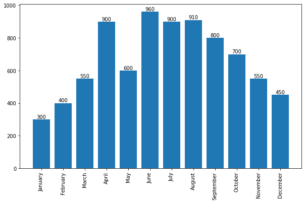
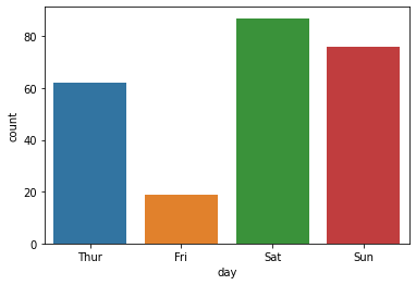
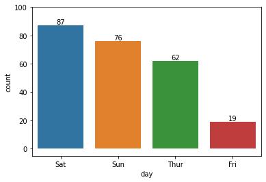
for plot in ax.patches: # matplotlib 와 같은 역할을 수행한다.
  print(plot)
  height = plot.get_height()
  ax.text(plot.get_x() + plot.get_width()/2., height, height, ha = 'center', va = 'bottom')  

ax.set_ylim(-5, 100)
plt.show()

Rectangle(xy=(-0.4, 0), width=0.8, height=87, angle=0)
Rectangle(xy=(0.6, 0), width=0.8, height=76, angle=0)
Rectangle(xy=(1.6, 0), width=0.8, height=62, angle=0)
Rectangle(xy=(2.6, 0), width=0.8, height=19, angle=0)

어려운 시각화 그래프

1
2
3
4
5
6
7
8
9
10
11
12
13
14
15
16
17
18
19
20
21
22
23
24
25
26
27
28
29
30
31
32
33
34
35
36
37
38
39
40
41
42
43
44
45
46
47
48
49
50
51
52
53
54
55
56
57
58
59
60
61
62
63
64
65
66
67
68
69
70
71
72

import matplotlib.pyplot as plt
import seaborn as sns
import numpy as np
from matplotlib.ticker import (MultipleLocator, AutoMinorLocator, FuncFormatter)

def major_formatter(x, pos):
  return "%.2f$" % x

formatter = FuncFormatter(major_formatter)

tips = sns.load_dataset("tips")
fig, ax = plt.subplots(nrows=1, ncols=2, figsize=(16, 6))


ax0 = sns.barplot(x="day", y="total_bill", data=tips,
            ci=None, color='lightgray', alpha=0.85, zorder=2,  # alpha는 투명도
            ax = ax[0])
# groupby
group_mean = tips.groupby(['day'])['total_bill'].agg('mean')
#print(group_mean)

h_day = group_mean.sort_values(ascending=False).index[0]  # sun 표시
#print(h_day)
h_mean = group_mean.sort_values(ascending=False).values[0]  
print(h_mean)

# text 추가
for plot in ax0.patches:
  height = np.round(plot.get_height(), 2)
  # print(height)

  # Default
  fontweight = "normal"
  color = "k"
  if h_mean == height:
    fontweight = "bold"
    color = "darkred"
    plot.set_facecolor(color)
    plot.set_edgecolor("black")

  ax0.text(plot.get_x() + plot.get_width()/2.,
           height + 1, height, 
           ha = 'center', size=12, fontweight = fontweight, color = color)

# 축 수정
ax0.set_ylim(-3, 30)
ax0.set_title("Bar Graph", size = 16)

# 테두리(spines) 삭제
ax0.spines['top'].set_visible(False)
ax0.spines['left'].set_position(("outward", 20))
ax0.spines['left'].set_visible(False)
ax0.spines['right'].set_visible(False)

ax0.yaxis.set_major_locator(MultipleLocator(10))
ax0.yaxis.set_major_formatter(formatter)
ax0.yaxis.set_minor_locator(MultipleLocator(5))

ax0.set_ylabel("Avg. Total Bill($)", fontsize=14)

ax0.grid(axis="y", which="major", color = "lightgray")
ax0.grid(axis="y", which="major", ls = ":")

for xtick in ax0.get_xticklabels():
  print(xtick)
  if xtick.get_text() == h_day:
    xtick.set_color("darkred")
    xtick.set_fontweight("demibold")

ax0.set_xticklabels(['Thursday', 'Friday', 'Saturday', 'Sunday'], size = 12)

plt.show()

21.41
Text(0, 0, 'Thur')
Text(0, 0, 'Fri')
Text(0, 0, 'Sat')
Text(0, 0, 'Sun')

• 라이브러리 불러오기

1
2

import pandas as pd
print(pd.__version__)

1.3.5

구글 드라이브 연동

• 구글 드라이브 → colab notebook → 새 폴더 생성 : data → 슬랙에서 다운 받은 lemonade.csv 파일을 올린다 -> 다음 코드를 실행

1
2

from google.colab import drive
drive.mount('/content/drive')

Mounted at /content/drive

Mounted at ..drive 가 출력되었으므로 성공

현재 좌측에 폴더 그림 -> drive -> mydrive -> Colab Notebooks -> data -> supermarket_sales.csv를 찾아서 우클릭 -> 경로 복사 -> 다음 코드에 붙여넣어 사용

1
2
3

DATA_PATH = '/content/drive/MyDrive/Colab Notebooks/data/supermarket_sales.csv'
sales = pd.read_csv(DATA_PATH)
sales

  <script>
    const buttonEl =
      document.querySelector('#df-8a1e46d8-83ea-49d2-a98d-cf274f10b34d button.colab-df-convert');
    buttonEl.style.display =
      google.colab.kernel.accessAllowed ? 'block' : 'none';

    async function convertToInteractive(key) {
      const element = document.querySelector('#df-8a1e46d8-83ea-49d2-a98d-cf274f10b34d');
      const dataTable =
        await google.colab.kernel.invokeFunction('convertToInteractive',
                                                 [key], {});
      if (!dataTable) return;

      const docLinkHtml = 'Like what you see? Visit the ' +
        '<a target="_blank" href=https://colab.research.google.com/notebooks/data_table.ipynb>data table notebook</a>'
        + ' to learn more about interactive tables.';
      element.innerHTML = '';
      dataTable['output_type'] = 'display_data';
      await google.colab.output.renderOutput(dataTable, element);
      const docLink = document.createElement('div');
      docLink.innerHTML = docLinkHtml;
      element.appendChild(docLink);
    }
  </script>
</div>

1

sales.info()

<class 'pandas.core.frame.DataFrame'>
RangeIndex: 1000 entries, 0 to 999
Data columns (total 11 columns):
 #   Column         Non-Null Count  Dtype  
---  ------         --------------  -----  
 0   Invoice ID     1000 non-null   object 
 1   Branch         1000 non-null   object 
 2   City           1000 non-null   object 
 3   Customer type  1000 non-null   object 
 4   Gender         1000 non-null   object 
 5   Product line   1000 non-null   object 
 6   Unit price     1000 non-null   float64
 7   Quantity       1000 non-null   int64  
 8   Date           1000 non-null   object 
 9   Time           1000 non-null   object 
 10  Payment        1000 non-null   object 
dtypes: float64(1), int64(1), object(9)
memory usage: 86.1+ KB

1
2

# 여러가지 시도해보면서 정보를 파악해보자
sales['Invoice ID'].value_counts()

750-67-8428    1
642-61-4706    1
816-72-8853    1
491-38-3499    1
322-02-2271    1
              ..
633-09-3463    1
374-17-3652    1
378-07-7001    1
433-75-6987    1
849-09-3807    1
Name: Invoice ID, Length: 1000, dtype: int64

1
2

# 여러가지 시도해보면서 정보를 파악해보자
sales.groupby('Customer type')['Quantity'].sum()

Customer type
Member    2785
Normal    2725
Name: Quantity, dtype: int64

1

sales.groupby(['Customer type', 'Branch', 'Payment'])['Quantity'].sum()

Customer type  Branch  Payment    
Member         A       Cash           308
                       Credit card    282
                       Ewallet        374
               B       Cash           284
                       Credit card    371
                       Ewallet        269
               C       Cash           293
                       Credit card    349
                       Ewallet        255
Normal         A       Cash           264
                       Credit card    298
                       Ewallet        333
               B       Cash           344
                       Credit card    228
                       Ewallet        324
               C       Cash           403
                       Credit card    194
                       Ewallet        337
Name: Quantity, dtype: int64

1

print(type(sales.groupby(['Customer type', 'Branch', 'Payment'])['Quantity'].sum()))

<class 'pandas.core.series.Series'>

1

sales.groupby(['Customer type', 'Branch', 'Payment'])['Quantity'].agg(['sum', 'mean'])

  <script>
    const buttonEl =
      document.querySelector('#df-9f19e00c-ea81-404c-b289-c9ddb325aeaa button.colab-df-convert');
    buttonEl.style.display =
      google.colab.kernel.accessAllowed ? 'block' : 'none';

    async function convertToInteractive(key) {
      const element = document.querySelector('#df-9f19e00c-ea81-404c-b289-c9ddb325aeaa');
      const dataTable =
        await google.colab.kernel.invokeFunction('convertToInteractive',
                                                 [key], {});
      if (!dataTable) return;

      const docLinkHtml = 'Like what you see? Visit the ' +
        '<a target="_blank" href=https://colab.research.google.com/notebooks/data_table.ipynb>data table notebook</a>'
        + ' to learn more about interactive tables.';
      element.innerHTML = '';
      dataTable['output_type'] = 'display_data';
      await google.colab.output.renderOutput(dataTable, element);
      const docLink = document.createElement('div');
      docLink.innerHTML = docLinkHtml;
      element.appendChild(docLink);
    }
  </script>
</div>

1

print(type(sales.groupby(['Customer type', 'Branch', 'Payment'])['Quantity'].agg(['sum', 'mean'])))

<class 'pandas.core.frame.DataFrame'>

1

sales.groupby(['Customer type', 'Branch', 'Payment'], as_index=False)['Quantity'].agg(['sum', 'mean'])

  <script>
    const buttonEl =
      document.querySelector('#df-f56f9b0d-43e2-4ba0-8abf-56fa96c5d20f button.colab-df-convert');
    buttonEl.style.display =
      google.colab.kernel.accessAllowed ? 'block' : 'none';

    async function convertToInteractive(key) {
      const element = document.querySelector('#df-f56f9b0d-43e2-4ba0-8abf-56fa96c5d20f');
      const dataTable =
        await google.colab.kernel.invokeFunction('convertToInteractive',
                                                 [key], {});
      if (!dataTable) return;

      const docLinkHtml = 'Like what you see? Visit the ' +
        '<a target="_blank" href=https://colab.research.google.com/notebooks/data_table.ipynb>data table notebook</a>'
        + ' to learn more about interactive tables.';
      element.innerHTML = '';
      dataTable['output_type'] = 'display_data';
      await google.colab.output.renderOutput(dataTable, element);
      const docLink = document.createElement('div');
      docLink.innerHTML = docLinkHtml;
      element.appendChild(docLink);
    }
  </script>
</div>

1
2
3
4
5
6
7
8
9
10
11

import pandas as pd
import numpy as np

dict_01 = {
    'Score_A' : [80, 90, np.nan, 80],
    'Score_B' : [30, 45, np.nan, np.nan],
    'Score_C' : [np.nan, 50, 80, 90],
}

df = pd.DataFrame(dict_01)
df

  <script>
    const buttonEl =
      document.querySelector('#df-6c9ddc3e-23cb-46c2-bcca-8e0adaab788b button.colab-df-convert');
    buttonEl.style.display =
      google.colab.kernel.accessAllowed ? 'block' : 'none';

    async function convertToInteractive(key) {
      const element = document.querySelector('#df-6c9ddc3e-23cb-46c2-bcca-8e0adaab788b');
      const dataTable =
        await google.colab.kernel.invokeFunction('convertToInteractive',
                                                 [key], {});
      if (!dataTable) return;

      const docLinkHtml = 'Like what you see? Visit the ' +
        '<a target="_blank" href=https://colab.research.google.com/notebooks/data_table.ipynb>data table notebook</a>'
        + ' to learn more about interactive tables.';
      element.innerHTML = '';
      dataTable['output_type'] = 'display_data';
      await google.colab.output.renderOutput(dataTable, element);
      const docLink = document.createElement('div');
      docLink.innerHTML = docLinkHtml;
      element.appendChild(docLink);
    }
  </script>
</div>

1

df.isnull().sum()

Score_A    1
Score_B    2
Score_C    1
dtype: int64

1

df.fillna("0")

  <script>
    const buttonEl =
      document.querySelector('#df-ce166771-c2da-430d-aa22-8b7cac811d94 button.colab-df-convert');
    buttonEl.style.display =
      google.colab.kernel.accessAllowed ? 'block' : 'none';

    async function convertToInteractive(key) {
      const element = document.querySelector('#df-ce166771-c2da-430d-aa22-8b7cac811d94');
      const dataTable =
        await google.colab.kernel.invokeFunction('convertToInteractive',
                                                 [key], {});
      if (!dataTable) return;

      const docLinkHtml = 'Like what you see? Visit the ' +
        '<a target="_blank" href=https://colab.research.google.com/notebooks/data_table.ipynb>data table notebook</a>'
        + ' to learn more about interactive tables.';
      element.innerHTML = '';
      dataTable['output_type'] = 'display_data';
      await google.colab.output.renderOutput(dataTable, element);
      const docLink = document.createElement('div');
      docLink.innerHTML = docLinkHtml;
      element.appendChild(docLink);
    }
  </script>
</div>

1
2

# 바로 윗칸의 데이터로 채우기
df.fillna(method="pad")

  <script>
    const buttonEl =
      document.querySelector('#df-14c34a17-7745-4466-a779-62f00b5030de button.colab-df-convert');
    buttonEl.style.display =
      google.colab.kernel.accessAllowed ? 'block' : 'none';

    async function convertToInteractive(key) {
      const element = document.querySelector('#df-14c34a17-7745-4466-a779-62f00b5030de');
      const dataTable =
        await google.colab.kernel.invokeFunction('convertToInteractive',
                                                 [key], {});
      if (!dataTable) return;

      const docLinkHtml = 'Like what you see? Visit the ' +
        '<a target="_blank" href=https://colab.research.google.com/notebooks/data_table.ipynb>data table notebook</a>'
        + ' to learn more about interactive tables.';
      element.innerHTML = '';
      dataTable['output_type'] = 'display_data';
      await google.colab.output.renderOutput(dataTable, element);
      const docLink = document.createElement('div');
      docLink.innerHTML = docLinkHtml;
      element.appendChild(docLink);
    }
  </script>
</div>

1
2
3
4
5
6
7

dict_01 = {
    "성별" : ["남자", "여자", np.nan, "남자"],
    "Salary" : [30, 45, 90, 70],
}

df = pd.DataFrame(dict_01)
df

  <script>
    const buttonEl =
      document.querySelector('#df-54d9e838-5824-4cb9-9f0f-8291411d9270 button.colab-df-convert');
    buttonEl.style.display =
      google.colab.kernel.accessAllowed ? 'block' : 'none';

    async function convertToInteractive(key) {
      const element = document.querySelector('#df-54d9e838-5824-4cb9-9f0f-8291411d9270');
      const dataTable =
        await google.colab.kernel.invokeFunction('convertToInteractive',
                                                 [key], {});
      if (!dataTable) return;

      const docLinkHtml = 'Like what you see? Visit the ' +
        '<a target="_blank" href=https://colab.research.google.com/notebooks/data_table.ipynb>data table notebook</a>'
        + ' to learn more about interactive tables.';
      element.innerHTML = '';
      dataTable['output_type'] = 'display_data';
      await google.colab.output.renderOutput(dataTable, element);
      const docLink = document.createElement('div');
      docLink.innerHTML = docLinkHtml;
      element.appendChild(docLink);
    }
  </script>
</div>

1

df['성별'].fillna("성별 없음")

0       남자
1       여자
2    성별 없음
3       남자
Name: 성별, dtype: object

1
2
3
4
5
6
7
8
9
10
11
12

import pandas as pd
import numpy as np

dict_01 = {
    'Score_A' : [80, 90, np.nan, 80],
    'Score_B' : [30, 45, np.nan, np.nan],
    'Score_C' : [np.nan, 50, 80, 90],
    'Score_D' : [50, 30, 80, 60],
}

df = pd.DataFrame(dict_01)
df

  <script>
    const buttonEl =
      document.querySelector('#df-a1c2a0ad-c902-4c13-8d35-ae4931ac7c3d button.colab-df-convert');
    buttonEl.style.display =
      google.colab.kernel.accessAllowed ? 'block' : 'none';

    async function convertToInteractive(key) {
      const element = document.querySelector('#df-a1c2a0ad-c902-4c13-8d35-ae4931ac7c3d');
      const dataTable =
        await google.colab.kernel.invokeFunction('convertToInteractive',
                                                 [key], {});
      if (!dataTable) return;

      const docLinkHtml = 'Like what you see? Visit the ' +
        '<a target="_blank" href=https://colab.research.google.com/notebooks/data_table.ipynb>data table notebook</a>'
        + ' to learn more about interactive tables.';
      element.innerHTML = '';
      dataTable['output_type'] = 'display_data';
      await google.colab.output.renderOutput(dataTable, element);
      const docLink = document.createElement('div');
      docLink.innerHTML = docLinkHtml;
      element.appendChild(docLink);
    }
  </script>
</div>

1

df.dropna(axis = 1)

  <script>
    const buttonEl =
      document.querySelector('#df-a9658aae-24a1-43bd-a6fe-73b30c752e90 button.colab-df-convert');
    buttonEl.style.display =
      google.colab.kernel.accessAllowed ? 'block' : 'none';

    async function convertToInteractive(key) {
      const element = document.querySelector('#df-a9658aae-24a1-43bd-a6fe-73b30c752e90');
      const dataTable =
        await google.colab.kernel.invokeFunction('convertToInteractive',
                                                 [key], {});
      if (!dataTable) return;

      const docLinkHtml = 'Like what you see? Visit the ' +
        '<a target="_blank" href=https://colab.research.google.com/notebooks/data_table.ipynb>data table notebook</a>'
        + ' to learn more about interactive tables.';
      element.innerHTML = '';
      dataTable['output_type'] = 'display_data';
      await google.colab.output.renderOutput(dataTable, element);
      const docLink = document.createElement('div');
      docLink.innerHTML = docLinkHtml;
      element.appendChild(docLink);
    }
  </script>
</div>

1

df.dropna(axis = 0)

  <script>
    const buttonEl =
      document.querySelector('#df-1359a925-a759-4d30-9b57-10abcaf3af1a button.colab-df-convert');
    buttonEl.style.display =
      google.colab.kernel.accessAllowed ? 'block' : 'none';

    async function convertToInteractive(key) {
      const element = document.querySelector('#df-1359a925-a759-4d30-9b57-10abcaf3af1a');
      const dataTable =
        await google.colab.kernel.invokeFunction('convertToInteractive',
                                                 [key], {});
      if (!dataTable) return;

      const docLinkHtml = 'Like what you see? Visit the ' +
        '<a target="_blank" href=https://colab.research.google.com/notebooks/data_table.ipynb>data table notebook</a>'
        + ' to learn more about interactive tables.';
      element.innerHTML = '';
      dataTable['output_type'] = 'display_data';
      await google.colab.output.renderOutput(dataTable, element);
      const docLink = document.createElement('div');
      docLink.innerHTML = docLinkHtml;
      element.appendChild(docLink);
    }
  </script>
</div>

1

sales

  <script>
    const buttonEl =
      document.querySelector('#df-04da7866-a736-4456-8d77-a7760df771c5 button.colab-df-convert');
    buttonEl.style.display =
      google.colab.kernel.accessAllowed ? 'block' : 'none';

    async function convertToInteractive(key) {
      const element = document.querySelector('#df-04da7866-a736-4456-8d77-a7760df771c5');
      const dataTable =
        await google.colab.kernel.invokeFunction('convertToInteractive',
                                                 [key], {});
      if (!dataTable) return;

      const docLinkHtml = 'Like what you see? Visit the ' +
        '<a target="_blank" href=https://colab.research.google.com/notebooks/data_table.ipynb>data table notebook</a>'
        + ' to learn more about interactive tables.';
      element.innerHTML = '';
      dataTable['output_type'] = 'display_data';
      await google.colab.output.renderOutput(dataTable, element);
      const docLink = document.createElement('div');
      docLink.innerHTML = docLinkHtml;
      element.appendChild(docLink);
    }
  </script>
</div>

1

sales[['Unit price']]. describe()

  <script>
    const buttonEl =
      document.querySelector('#df-6bdae016-4a2d-4f55-9e51-5f68e6af7217 button.colab-df-convert');
    buttonEl.style.display =
      google.colab.kernel.accessAllowed ? 'block' : 'none';

    async function convertToInteractive(key) {
      const element = document.querySelector('#df-6bdae016-4a2d-4f55-9e51-5f68e6af7217');
      const dataTable =
        await google.colab.kernel.invokeFunction('convertToInteractive',
                                                 [key], {});
      if (!dataTable) return;

      const docLinkHtml = 'Like what you see? Visit the ' +
        '<a target="_blank" href=https://colab.research.google.com/notebooks/data_table.ipynb>data table notebook</a>'
        + ' to learn more about interactive tables.';
      element.innerHTML = '';
      dataTable['output_type'] = 'display_data';
      await google.colab.output.renderOutput(dataTable, element);
      const docLink = document.createElement('div');
      docLink.innerHTML = docLinkHtml;
      element.appendChild(docLink);
    }
  </script>
</div>

1
2
3
4
5
6
7
8

Q1 = sales['Unit price'].quantile(0.25)
Q3 = sales['Unit price'].quantile(0.75)

# Q1보다 낮은 값을 이상치로 간주
outliers_q1 = (sales['Unit price'] < Q1)

# Q1보다 높은 값을 이상치로 간주
outliers_q3 = (sales['Unit price'] > Q3)

1

print(sales['Unit price'][~(outliers_q1 | outliers_q3)])

0      74.69
2      46.33
3      58.22
6      68.84
7      73.56
       ...  
991    76.60
992    58.03
994    60.95
995    40.35
998    65.82
Name: Unit price, Length: 500, dtype: float64

Pandas 10분 완성

https://dataitgirls2.github.io/10minutes2pandas/

1
2
3
4

# 라이브러리 불러오기
import pandas as pd
import numpy as np
import matplotlib.pyplot as plt

1.Object Creation (객체 생성)

• Pandas는 값을 가지고 있는 리스트를 통해 Series를 만들고, 정수로 만들어진 인덱스를 기본값으로 불러온다.

1
2
3

# Series를 이용한 객체 생성
s = pd.Series([1,3,5,np.nan,6,8])
s

0    1.0
1    3.0
2    5.0
3    NaN
4    6.0
5    8.0
dtype: float64

• datetime 인덱스와 레이블이 있는 열을 가지고 있는 numpy 배열을 전달하여 데이터프레임을 만든다.

1
2
3

# date_range()를 이용해 20130101을 포함한 연속적인 6일의 데이터를 넣는다.
dates = pd.date_range('20130101', periods = 6)
dates

DatetimeIndex(['2013-01-01', '2013-01-02', '2013-01-03', '2013-01-04',
               '2013-01-05', '2013-01-06'],
              dtype='datetime64[ns]', freq='D')

1
2
3

# 데이터 프레임 생성
df = pd.DataFrame(np.random.randn(6,4), index=dates, columns=list('ABCD'))
df

  <script>
    const buttonEl =
      document.querySelector('#df-98ec8384-9a3f-4ee3-9d62-d8f6d1821857 button.colab-df-convert');
    buttonEl.style.display =
      google.colab.kernel.accessAllowed ? 'block' : 'none';

    async function convertToInteractive(key) {
      const element = document.querySelector('#df-98ec8384-9a3f-4ee3-9d62-d8f6d1821857');
      const dataTable =
        await google.colab.kernel.invokeFunction('convertToInteractive',
                                                 [key], {});
      if (!dataTable) return;

      const docLinkHtml = 'Like what you see? Visit the ' +
        '<a target="_blank" href=https://colab.research.google.com/notebooks/data_table.ipynb>data table notebook</a>'
        + ' to learn more about interactive tables.';
      element.innerHTML = '';
      dataTable['output_type'] = 'display_data';
      await google.colab.output.renderOutput(dataTable, element);
      const docLink = document.createElement('div');
      docLink.innerHTML = docLinkHtml;
      element.appendChild(docLink);
    }
  </script>
</div>

1
2
3
4
5
6
7
8

df2 = pd.DataFrame({'A' : 1.,
                    'B' : pd.Timestamp('20130102'),
                    'C' : pd.Series(1, index=list(range(4)), dtype='float32'),
                    'D' : np.array([3] * 4,dtype = 'int32'),
                    'E' : pd.Categorical(["test", "train", "test", "train"]),
                    'F' : 'foo'})

df2

  <script>
    const buttonEl =
      document.querySelector('#df-32a9a2b4-301b-48af-8afa-569444b4838a button.colab-df-convert');
    buttonEl.style.display =
      google.colab.kernel.accessAllowed ? 'block' : 'none';

    async function convertToInteractive(key) {
      const element = document.querySelector('#df-32a9a2b4-301b-48af-8afa-569444b4838a');
      const dataTable =
        await google.colab.kernel.invokeFunction('convertToInteractive',
                                                 [key], {});
      if (!dataTable) return;

      const docLinkHtml = 'Like what you see? Visit the ' +
        '<a target="_blank" href=https://colab.research.google.com/notebooks/data_table.ipynb>data table notebook</a>'
        + ' to learn more about interactive tables.';
      element.innerHTML = '';
      dataTable['output_type'] = 'display_data';
      await google.colab.output.renderOutput(dataTable, element);
      const docLink = document.createElement('div');
      docLink.innerHTML = docLinkHtml;
      element.appendChild(docLink);
    }
  </script>
</div>

1

df2.dtypes

A           float64
B    datetime64[ns]
C           float32
D             int32
E          category
F            object
dtype: object

1
2

df.tail(3)  # 끝에서부터 3줄을 출력
df.tail()   # 끝에서부터 5줄을 출력. 디폴트값이 5이다

  <script>
    const buttonEl =
      document.querySelector('#df-b90adfec-6c56-41b4-a15c-699d26a51033 button.colab-df-convert');
    buttonEl.style.display =
      google.colab.kernel.accessAllowed ? 'block' : 'none';

    async function convertToInteractive(key) {
      const element = document.querySelector('#df-b90adfec-6c56-41b4-a15c-699d26a51033');
      const dataTable =
        await google.colab.kernel.invokeFunction('convertToInteractive',
                                                 [key], {});
      if (!dataTable) return;

      const docLinkHtml = 'Like what you see? Visit the ' +
        '<a target="_blank" href=https://colab.research.google.com/notebooks/data_table.ipynb>data table notebook</a>'
        + ' to learn more about interactive tables.';
      element.innerHTML = '';
      dataTable['output_type'] = 'display_data';
      await google.colab.output.renderOutput(dataTable, element);
      const docLink = document.createElement('div');
      docLink.innerHTML = docLinkHtml;
      element.appendChild(docLink);
    }
  </script>
</div>

1

df.head() # 처음 5줄을 출력.

  <script>
    const buttonEl =
      document.querySelector('#df-1d5aaccf-3123-46cc-a71a-b7f235656a2f button.colab-df-convert');
    buttonEl.style.display =
      google.colab.kernel.accessAllowed ? 'block' : 'none';

    async function convertToInteractive(key) {
      const element = document.querySelector('#df-1d5aaccf-3123-46cc-a71a-b7f235656a2f');
      const dataTable =
        await google.colab.kernel.invokeFunction('convertToInteractive',
                                                 [key], {});
      if (!dataTable) return;

      const docLinkHtml = 'Like what you see? Visit the ' +
        '<a target="_blank" href=https://colab.research.google.com/notebooks/data_table.ipynb>data table notebook</a>'
        + ' to learn more about interactive tables.';
      element.innerHTML = '';
      dataTable['output_type'] = 'display_data';
      await google.colab.output.renderOutput(dataTable, element);
      const docLink = document.createElement('div');
      docLink.innerHTML = docLinkHtml;
      element.appendChild(docLink);
    }
  </script>
</div>

1

df.index

DatetimeIndex(['2013-01-01', '2013-01-02', '2013-01-03', '2013-01-04',
               '2013-01-05', '2013-01-06'],
              dtype='datetime64[ns]', freq='D')

1

df.columns

Index(['A', 'B', 'C', 'D'], dtype='object')

1

df.values

array([[-0.21437119, -0.48933404,  0.80787593, -2.32856993],
       [-0.01876194, -0.43804563,  0.59387975,  0.67184854],
       [-0.59620717,  0.08161493,  0.18211706, -2.06300731],
       [-2.0447528 , -0.85342539,  1.58247067, -0.75623263],
       [ 0.39497306, -0.52676189,  0.39385602,  1.55066002],
       [-1.66587853,  0.18490331,  1.9057098 ,  2.34549952]])

1

df.describe()

  <script>
    const buttonEl =
      document.querySelector('#df-bc50d2c1-8824-4181-b8ce-c7aecf4a30e1 button.colab-df-convert');
    buttonEl.style.display =
      google.colab.kernel.accessAllowed ? 'block' : 'none';

    async function convertToInteractive(key) {
      const element = document.querySelector('#df-bc50d2c1-8824-4181-b8ce-c7aecf4a30e1');
      const dataTable =
        await google.colab.kernel.invokeFunction('convertToInteractive',
                                                 [key], {});
      if (!dataTable) return;

      const docLinkHtml = 'Like what you see? Visit the ' +
        '<a target="_blank" href=https://colab.research.google.com/notebooks/data_table.ipynb>data table notebook</a>'
        + ' to learn more about interactive tables.';
      element.innerHTML = '';
      dataTable['output_type'] = 'display_data';
      await google.colab.output.renderOutput(dataTable, element);
      const docLink = document.createElement('div');
      docLink.innerHTML = docLinkHtml;
      element.appendChild(docLink);
    }
  </script>
</div>

1

df.T

  <script>
    const buttonEl =
      document.querySelector('#df-cfc48a53-c108-4b41-bf62-f85fc6923d20 button.colab-df-convert');
    buttonEl.style.display =
      google.colab.kernel.accessAllowed ? 'block' : 'none';

    async function convertToInteractive(key) {
      const element = document.querySelector('#df-cfc48a53-c108-4b41-bf62-f85fc6923d20');
      const dataTable =
        await google.colab.kernel.invokeFunction('convertToInteractive',
                                                 [key], {});
      if (!dataTable) return;

      const docLinkHtml = 'Like what you see? Visit the ' +
        '<a target="_blank" href=https://colab.research.google.com/notebooks/data_table.ipynb>data table notebook</a>'
        + ' to learn more about interactive tables.';
      element.innerHTML = '';
      dataTable['output_type'] = 'display_data';
      await google.colab.output.renderOutput(dataTable, element);
      const docLink = document.createElement('div');
      docLink.innerHTML = docLinkHtml;
      element.appendChild(docLink);
    }
  </script>
</div>

1
2

df.sort_index(axis=1, ascending=False)
# axis=1 일때, 열방향으로 실행한다.

  <script>
    const buttonEl =
      document.querySelector('#df-2b34e281-4cce-48fe-b140-c57dc7828ca4 button.colab-df-convert');
    buttonEl.style.display =
      google.colab.kernel.accessAllowed ? 'block' : 'none';

    async function convertToInteractive(key) {
      const element = document.querySelector('#df-2b34e281-4cce-48fe-b140-c57dc7828ca4');
      const dataTable =
        await google.colab.kernel.invokeFunction('convertToInteractive',
                                                 [key], {});
      if (!dataTable) return;

      const docLinkHtml = 'Like what you see? Visit the ' +
        '<a target="_blank" href=https://colab.research.google.com/notebooks/data_table.ipynb>data table notebook</a>'
        + ' to learn more about interactive tables.';
      element.innerHTML = '';
      dataTable['output_type'] = 'display_data';
      await google.colab.output.renderOutput(dataTable, element);
      const docLink = document.createElement('div');
      docLink.innerHTML = docLinkHtml;
      element.appendChild(docLink);
    }
  </script>
</div>

1

df.sort_values(by='B')

  <script>
    const buttonEl =
      document.querySelector('#df-30e7da7b-4a36-43a6-b2c3-a5a382f252de button.colab-df-convert');
    buttonEl.style.display =
      google.colab.kernel.accessAllowed ? 'block' : 'none';

    async function convertToInteractive(key) {
      const element = document.querySelector('#df-30e7da7b-4a36-43a6-b2c3-a5a382f252de');
      const dataTable =
        await google.colab.kernel.invokeFunction('convertToInteractive',
                                                 [key], {});
      if (!dataTable) return;

      const docLinkHtml = 'Like what you see? Visit the ' +
        '<a target="_blank" href=https://colab.research.google.com/notebooks/data_table.ipynb>data table notebook</a>'
        + ' to learn more about interactive tables.';
      element.innerHTML = '';
      dataTable['output_type'] = 'display_data';
      await google.colab.output.renderOutput(dataTable, element);
      const docLink = document.createElement('div');
      docLink.innerHTML = docLinkHtml;
      element.appendChild(docLink);
    }
  </script>
</div>

1

df['A']

2013-01-01   -0.214371
2013-01-02   -0.018762
2013-01-03   -0.596207
2013-01-04   -2.044753
2013-01-05    0.394973
2013-01-06   -1.665879
Freq: D, Name: A, dtype: float64

1

df[0:3]

  <script>
    const buttonEl =
      document.querySelector('#df-42a08968-1f35-45a3-bca9-318f73f513c6 button.colab-df-convert');
    buttonEl.style.display =
      google.colab.kernel.accessAllowed ? 'block' : 'none';

    async function convertToInteractive(key) {
      const element = document.querySelector('#df-42a08968-1f35-45a3-bca9-318f73f513c6');
      const dataTable =
        await google.colab.kernel.invokeFunction('convertToInteractive',
                                                 [key], {});
      if (!dataTable) return;

      const docLinkHtml = 'Like what you see? Visit the ' +
        '<a target="_blank" href=https://colab.research.google.com/notebooks/data_table.ipynb>data table notebook</a>'
        + ' to learn more about interactive tables.';
      element.innerHTML = '';
      dataTable['output_type'] = 'display_data';
      await google.colab.output.renderOutput(dataTable, element);
      const docLink = document.createElement('div');
      docLink.innerHTML = docLinkHtml;
      element.appendChild(docLink);
    }
  </script>
</div>

1

df['20130102':'20130104']

  <script>
    const buttonEl =
      document.querySelector('#df-ebb43e9b-1f8f-4438-93a1-e004bc46108e button.colab-df-convert');
    buttonEl.style.display =
      google.colab.kernel.accessAllowed ? 'block' : 'none';

    async function convertToInteractive(key) {
      const element = document.querySelector('#df-ebb43e9b-1f8f-4438-93a1-e004bc46108e');
      const dataTable =
        await google.colab.kernel.invokeFunction('convertToInteractive',
                                                 [key], {});
      if (!dataTable) return;

      const docLinkHtml = 'Like what you see? Visit the ' +
        '<a target="_blank" href=https://colab.research.google.com/notebooks/data_table.ipynb>data table notebook</a>'
        + ' to learn more about interactive tables.';
      element.innerHTML = '';
      dataTable['output_type'] = 'display_data';
      await google.colab.output.renderOutput(dataTable, element);
      const docLink = document.createElement('div');
      docLink.innerHTML = docLinkHtml;
      element.appendChild(docLink);
    }
  </script>
</div>

1

df.loc[dates[0]]

A   -0.214371
B   -0.489334
C    0.807876
D   -2.328570
Name: 2013-01-01 00:00:00, dtype: float64

1

df.loc[:,['A','B']]

  <script>
    const buttonEl =
      document.querySelector('#df-0d130634-6f70-4a3b-a931-3907cbf47eb6 button.colab-df-convert');
    buttonEl.style.display =
      google.colab.kernel.accessAllowed ? 'block' : 'none';

    async function convertToInteractive(key) {
      const element = document.querySelector('#df-0d130634-6f70-4a3b-a931-3907cbf47eb6');
      const dataTable =
        await google.colab.kernel.invokeFunction('convertToInteractive',
                                                 [key], {});
      if (!dataTable) return;

      const docLinkHtml = 'Like what you see? Visit the ' +
        '<a target="_blank" href=https://colab.research.google.com/notebooks/data_table.ipynb>data table notebook</a>'
        + ' to learn more about interactive tables.';
      element.innerHTML = '';
      dataTable['output_type'] = 'display_data';
      await google.colab.output.renderOutput(dataTable, element);
      const docLink = document.createElement('div');
      docLink.innerHTML = docLinkHtml;
      element.appendChild(docLink);
    }
  </script>
</div>

1

df.loc['20130102':'20130104', ['A','B']]

  <script>
    const buttonEl =
      document.querySelector('#df-80998ed9-78c8-48ef-84e6-b2e58d3420c3 button.colab-df-convert');
    buttonEl.style.display =
      google.colab.kernel.accessAllowed ? 'block' : 'none';

    async function convertToInteractive(key) {
      const element = document.querySelector('#df-80998ed9-78c8-48ef-84e6-b2e58d3420c3');
      const dataTable =
        await google.colab.kernel.invokeFunction('convertToInteractive',
                                                 [key], {});
      if (!dataTable) return;

      const docLinkHtml = 'Like what you see? Visit the ' +
        '<a target="_blank" href=https://colab.research.google.com/notebooks/data_table.ipynb>data table notebook</a>'
        + ' to learn more about interactive tables.';
      element.innerHTML = '';
      dataTable['output_type'] = 'display_data';
      await google.colab.output.renderOutput(dataTable, element);
      const docLink = document.createElement('div');
      docLink.innerHTML = docLinkHtml;
      element.appendChild(docLink);
    }
  </script>
</div>

1

df.loc['20130102',['A','B']]

A   -0.018762
B   -0.438046
Name: 2013-01-02 00:00:00, dtype: float64

1

df.loc[dates[0], 'A']

-0.21437119207750993

1

df.at[dates[0], 'A']

-0.21437119207750993

1

df.iloc[3]

A   -2.044753
B   -0.853425
C    1.582471
D   -0.756233
Name: 2013-01-04 00:00:00, dtype: float64

1

df.iloc[3:5, 0:2]

  <script>
    const buttonEl =
      document.querySelector('#df-a6c9e7cd-47c2-42bc-8726-b9b8dbf72bb9 button.colab-df-convert');
    buttonEl.style.display =
      google.colab.kernel.accessAllowed ? 'block' : 'none';

    async function convertToInteractive(key) {
      const element = document.querySelector('#df-a6c9e7cd-47c2-42bc-8726-b9b8dbf72bb9');
      const dataTable =
        await google.colab.kernel.invokeFunction('convertToInteractive',
                                                 [key], {});
      if (!dataTable) return;

      const docLinkHtml = 'Like what you see? Visit the ' +
        '<a target="_blank" href=https://colab.research.google.com/notebooks/data_table.ipynb>data table notebook</a>'
        + ' to learn more about interactive tables.';
      element.innerHTML = '';
      dataTable['output_type'] = 'display_data';
      await google.colab.output.renderOutput(dataTable, element);
      const docLink = document.createElement('div');
      docLink.innerHTML = docLinkHtml;
      element.appendChild(docLink);
    }
  </script>
</div>

1

df.iloc[[1, 2, 4], [0, 2]]

  <script>
    const buttonEl =
      document.querySelector('#df-1d8279d9-f642-48e7-8d6a-5006bade95b3 button.colab-df-convert');
    buttonEl.style.display =
      google.colab.kernel.accessAllowed ? 'block' : 'none';

    async function convertToInteractive(key) {
      const element = document.querySelector('#df-1d8279d9-f642-48e7-8d6a-5006bade95b3');
      const dataTable =
        await google.colab.kernel.invokeFunction('convertToInteractive',
                                                 [key], {});
      if (!dataTable) return;

      const docLinkHtml = 'Like what you see? Visit the ' +
        '<a target="_blank" href=https://colab.research.google.com/notebooks/data_table.ipynb>data table notebook</a>'
        + ' to learn more about interactive tables.';
      element.innerHTML = '';
      dataTable['output_type'] = 'display_data';
      await google.colab.output.renderOutput(dataTable, element);
      const docLink = document.createElement('div');
      docLink.innerHTML = docLinkHtml;
      element.appendChild(docLink);
    }
  </script>
</div>

1

df.iloc[1:3, : ]

  <script>
    const buttonEl =
      document.querySelector('#df-f8cec5e2-bbc6-4151-9e24-a55e5e4cd2b8 button.colab-df-convert');
    buttonEl.style.display =
      google.colab.kernel.accessAllowed ? 'block' : 'none';

    async function convertToInteractive(key) {
      const element = document.querySelector('#df-f8cec5e2-bbc6-4151-9e24-a55e5e4cd2b8');
      const dataTable =
        await google.colab.kernel.invokeFunction('convertToInteractive',
                                                 [key], {});
      if (!dataTable) return;

      const docLinkHtml = 'Like what you see? Visit the ' +
        '<a target="_blank" href=https://colab.research.google.com/notebooks/data_table.ipynb>data table notebook</a>'
        + ' to learn more about interactive tables.';
      element.innerHTML = '';
      dataTable['output_type'] = 'display_data';
      await google.colab.output.renderOutput(dataTable, element);
      const docLink = document.createElement('div');
      docLink.innerHTML = docLinkHtml;
      element.appendChild(docLink);
    }
  </script>
</div>

1

df.iloc[ : , 1:3]

  <script>
    const buttonEl =
      document.querySelector('#df-e2e93a02-91f2-43f7-a503-bec4339b83b8 button.colab-df-convert');
    buttonEl.style.display =
      google.colab.kernel.accessAllowed ? 'block' : 'none';

    async function convertToInteractive(key) {
      const element = document.querySelector('#df-e2e93a02-91f2-43f7-a503-bec4339b83b8');
      const dataTable =
        await google.colab.kernel.invokeFunction('convertToInteractive',
                                                 [key], {});
      if (!dataTable) return;

      const docLinkHtml = 'Like what you see? Visit the ' +
        '<a target="_blank" href=https://colab.research.google.com/notebooks/data_table.ipynb>data table notebook</a>'
        + ' to learn more about interactive tables.';
      element.innerHTML = '';
      dataTable['output_type'] = 'display_data';
      await google.colab.output.renderOutput(dataTable, element);
      const docLink = document.createElement('div');
      docLink.innerHTML = docLinkHtml;
      element.appendChild(docLink);
    }
  </script>
</div>

1

df.iloc[1, 1]

-0.43804562902186034

1

df.iat[1,1]

-0.43804562902186034

1

df[df.A > 0]

  <script>
    const buttonEl =
      document.querySelector('#df-4f4aed32-1929-4051-a6c9-8f593fb92c84 button.colab-df-convert');
    buttonEl.style.display =
      google.colab.kernel.accessAllowed ? 'block' : 'none';

    async function convertToInteractive(key) {
      const element = document.querySelector('#df-4f4aed32-1929-4051-a6c9-8f593fb92c84');
      const dataTable =
        await google.colab.kernel.invokeFunction('convertToInteractive',
                                                 [key], {});
      if (!dataTable) return;

      const docLinkHtml = 'Like what you see? Visit the ' +
        '<a target="_blank" href=https://colab.research.google.com/notebooks/data_table.ipynb>data table notebook</a>'
        + ' to learn more about interactive tables.';
      element.innerHTML = '';
      dataTable['output_type'] = 'display_data';
      await google.colab.output.renderOutput(dataTable, element);
      const docLink = document.createElement('div');
      docLink.innerHTML = docLinkHtml;
      element.appendChild(docLink);
    }
  </script>
</div>

1

df[df > 0]

  <script>
    const buttonEl =
      document.querySelector('#df-35a1e446-5c1c-4a6c-b39d-6ff2b7801761 button.colab-df-convert');
    buttonEl.style.display =
      google.colab.kernel.accessAllowed ? 'block' : 'none';

    async function convertToInteractive(key) {
      const element = document.querySelector('#df-35a1e446-5c1c-4a6c-b39d-6ff2b7801761');
      const dataTable =
        await google.colab.kernel.invokeFunction('convertToInteractive',
                                                 [key], {});
      if (!dataTable) return;

      const docLinkHtml = 'Like what you see? Visit the ' +
        '<a target="_blank" href=https://colab.research.google.com/notebooks/data_table.ipynb>data table notebook</a>'
        + ' to learn more about interactive tables.';
      element.innerHTML = '';
      dataTable['output_type'] = 'display_data';
      await google.colab.output.renderOutput(dataTable, element);
      const docLink = document.createElement('div');
      docLink.innerHTML = docLinkHtml;
      element.appendChild(docLink);
    }
  </script>
</div>

1
2
3

df2 = df.copy()
df2 = ['one', 'one', 'two', 'three', 'four', 'three']
df2

1

# df2[df2['E'].isin(['two','four'])]

1
2

s1 = pd.Series([1,2,3,4,5,6], index=pd.date_range('20130102', periods=6))
s1

2013-01-02    1
2013-01-03    2
2013-01-04    3
2013-01-05    4
2013-01-06    5
2013-01-07    6
Freq: D, dtype: int64

1

df['F'] = s1

1

df.at[dates[0], 'A'] = 0

1

df.iat[0, 1] = 0

1

df.loc[:, 'D'] = np.array([5] * len(df))

1

df

  <script>
    const buttonEl =
      document.querySelector('#df-12bdced2-022e-4cec-87a4-12165a361bd7 button.colab-df-convert');
    buttonEl.style.display =
      google.colab.kernel.accessAllowed ? 'block' : 'none';

    async function convertToInteractive(key) {
      const element = document.querySelector('#df-12bdced2-022e-4cec-87a4-12165a361bd7');
      const dataTable =
        await google.colab.kernel.invokeFunction('convertToInteractive',
                                                 [key], {});
      if (!dataTable) return;

      const docLinkHtml = 'Like what you see? Visit the ' +
        '<a target="_blank" href=https://colab.research.google.com/notebooks/data_table.ipynb>data table notebook</a>'
        + ' to learn more about interactive tables.';
      element.innerHTML = '';
      dataTable['output_type'] = 'display_data';
      await google.colab.output.renderOutput(dataTable, element);
      const docLink = document.createElement('div');
      docLink.innerHTML = docLinkHtml;
      element.appendChild(docLink);
    }
  </script>
</div>

1
2
3

df2 = df.copy()
df2[df2 > 0] = -df2
df2

  <script>
    const buttonEl =
      document.querySelector('#df-2e3a7cd9-4958-46ba-a9ca-9fb4031816c0 button.colab-df-convert');
    buttonEl.style.display =
      google.colab.kernel.accessAllowed ? 'block' : 'none';

    async function convertToInteractive(key) {
      const element = document.querySelector('#df-2e3a7cd9-4958-46ba-a9ca-9fb4031816c0');
      const dataTable =
        await google.colab.kernel.invokeFunction('convertToInteractive',
                                                 [key], {});
      if (!dataTable) return;

      const docLinkHtml = 'Like what you see? Visit the ' +
        '<a target="_blank" href=https://colab.research.google.com/notebooks/data_table.ipynb>data table notebook</a>'
        + ' to learn more about interactive tables.';
      element.innerHTML = '';
      dataTable['output_type'] = 'display_data';
      await google.colab.output.renderOutput(dataTable, element);
      const docLink = document.createElement('div');
      docLink.innerHTML = docLinkHtml;
      element.appendChild(docLink);
    }
  </script>
</div>

1
2
3

df1 = df.reindex(index=dates[0:4], columns=list(df.columns) + ['E'])
df1.loc[dates[0]:dates[1], 'E'] = 1
df1

  <script>
    const buttonEl =
      document.querySelector('#df-bd5a580c-316a-44a4-b5af-496ed1ad2f48 button.colab-df-convert');
    buttonEl.style.display =
      google.colab.kernel.accessAllowed ? 'block' : 'none';

    async function convertToInteractive(key) {
      const element = document.querySelector('#df-bd5a580c-316a-44a4-b5af-496ed1ad2f48');
      const dataTable =
        await google.colab.kernel.invokeFunction('convertToInteractive',
                                                 [key], {});
      if (!dataTable) return;

      const docLinkHtml = 'Like what you see? Visit the ' +
        '<a target="_blank" href=https://colab.research.google.com/notebooks/data_table.ipynb>data table notebook</a>'
        + ' to learn more about interactive tables.';
      element.innerHTML = '';
      dataTable['output_type'] = 'display_data';
      await google.colab.output.renderOutput(dataTable, element);
      const docLink = document.createElement('div');
      docLink.innerHTML = docLinkHtml;
      element.appendChild(docLink);
    }
  </script>
</div>

1

df1.dropna(how = 'any')

  <script>
    const buttonEl =
      document.querySelector('#df-e2491041-b1d4-4902-9dce-0ef94792d204 button.colab-df-convert');
    buttonEl.style.display =
      google.colab.kernel.accessAllowed ? 'block' : 'none';

    async function convertToInteractive(key) {
      const element = document.querySelector('#df-e2491041-b1d4-4902-9dce-0ef94792d204');
      const dataTable =
        await google.colab.kernel.invokeFunction('convertToInteractive',
                                                 [key], {});
      if (!dataTable) return;

      const docLinkHtml = 'Like what you see? Visit the ' +
        '<a target="_blank" href=https://colab.research.google.com/notebooks/data_table.ipynb>data table notebook</a>'
        + ' to learn more about interactive tables.';
      element.innerHTML = '';
      dataTable['output_type'] = 'display_data';
      await google.colab.output.renderOutput(dataTable, element);
      const docLink = document.createElement('div');
      docLink.innerHTML = docLinkHtml;
      element.appendChild(docLink);
    }
  </script>
</div>

1

df1.fillna(value=5)

  <script>
    const buttonEl =
      document.querySelector('#df-d9ef038f-e4ba-4702-b903-2a4056ec371e button.colab-df-convert');
    buttonEl.style.display =
      google.colab.kernel.accessAllowed ? 'block' : 'none';

    async function convertToInteractive(key) {
      const element = document.querySelector('#df-d9ef038f-e4ba-4702-b903-2a4056ec371e');
      const dataTable =
        await google.colab.kernel.invokeFunction('convertToInteractive',
                                                 [key], {});
      if (!dataTable) return;

      const docLinkHtml = 'Like what you see? Visit the ' +
        '<a target="_blank" href=https://colab.research.google.com/notebooks/data_table.ipynb>data table notebook</a>'
        + ' to learn more about interactive tables.';
      element.innerHTML = '';
      dataTable['output_type'] = 'display_data';
      await google.colab.output.renderOutput(dataTable, element);
      const docLink = document.createElement('div');
      docLink.innerHTML = docLinkHtml;
      element.appendChild(docLink);
    }
  </script>
</div>

1

pd.isna(df1)

  <script>
    const buttonEl =
      document.querySelector('#df-5ac60ecc-0098-4e10-8e23-74a0aa20e121 button.colab-df-convert');
    buttonEl.style.display =
      google.colab.kernel.accessAllowed ? 'block' : 'none';

    async function convertToInteractive(key) {
      const element = document.querySelector('#df-5ac60ecc-0098-4e10-8e23-74a0aa20e121');
      const dataTable =
        await google.colab.kernel.invokeFunction('convertToInteractive',
                                                 [key], {});
      if (!dataTable) return;

      const docLinkHtml = 'Like what you see? Visit the ' +
        '<a target="_blank" href=https://colab.research.google.com/notebooks/data_table.ipynb>data table notebook</a>'
        + ' to learn more about interactive tables.';
      element.innerHTML = '';
      dataTable['output_type'] = 'display_data';
      await google.colab.output.renderOutput(dataTable, element);
      const docLink = document.createElement('div');
      docLink.innerHTML = docLinkHtml;
      element.appendChild(docLink);
    }
  </script>
</div>

1

df.mean()

A   -0.655105
B   -0.258619
C    0.910985
D    5.000000
F    3.000000
dtype: float64

1

df.mean(1)

2013-01-01    1.451969
2013-01-02    1.227414
2013-01-03    1.333505
2013-01-04    1.336858
2013-01-05    1.852413
2013-01-06    2.084947
Freq: D, dtype: float64

1
2

s = pd.Series([1, 3, 4, np.nan, 6, 8], index=dates)
s

2013-01-01    1.0
2013-01-02    3.0
2013-01-03    4.0
2013-01-04    NaN
2013-01-05    6.0
2013-01-06    8.0
Freq: D, dtype: float64

1
2

s = pd.Series([1, 3, 4, np.nan, 6, 8], index=dates).shift(2)
s

2013-01-01    NaN
2013-01-02    NaN
2013-01-03    1.0
2013-01-04    3.0
2013-01-05    4.0
2013-01-06    NaN
Freq: D, dtype: float64

1

df.sub(s, axis='index')   

  <script>
    const buttonEl =
      document.querySelector('#df-99b442a2-cd95-4ff7-886d-18b60cfb80eb button.colab-df-convert');
    buttonEl.style.display =
      google.colab.kernel.accessAllowed ? 'block' : 'none';

    async function convertToInteractive(key) {
      const element = document.querySelector('#df-99b442a2-cd95-4ff7-886d-18b60cfb80eb');
      const dataTable =
        await google.colab.kernel.invokeFunction('convertToInteractive',
                                                 [key], {});
      if (!dataTable) return;

      const docLinkHtml = 'Like what you see? Visit the ' +
        '<a target="_blank" href=https://colab.research.google.com/notebooks/data_table.ipynb>data table notebook</a>'
        + ' to learn more about interactive tables.';
      element.innerHTML = '';
      dataTable['output_type'] = 'display_data';
      await google.colab.output.renderOutput(dataTable, element);
      const docLink = document.createElement('div');
      docLink.innerHTML = docLinkHtml;
      element.appendChild(docLink);
    }
  </script>
</div>

1

df.apply(np.cumsum)

  <script>
    const buttonEl =
      document.querySelector('#df-5f71bb31-515e-4d3e-b14d-f49a6239f43b button.colab-df-convert');
    buttonEl.style.display =
      google.colab.kernel.accessAllowed ? 'block' : 'none';

    async function convertToInteractive(key) {
      const element = document.querySelector('#df-5f71bb31-515e-4d3e-b14d-f49a6239f43b');
      const dataTable =
        await google.colab.kernel.invokeFunction('convertToInteractive',
                                                 [key], {});
      if (!dataTable) return;

      const docLinkHtml = 'Like what you see? Visit the ' +
        '<a target="_blank" href=https://colab.research.google.com/notebooks/data_table.ipynb>data table notebook</a>'
        + ' to learn more about interactive tables.';
      element.innerHTML = '';
      dataTable['output_type'] = 'display_data';
      await google.colab.output.renderOutput(dataTable, element);
      const docLink = document.createElement('div');
      docLink.innerHTML = docLinkHtml;
      element.appendChild(docLink);
    }
  </script>
</div>

1

df.apply(lambda x: x.max() - x.min())

A    2.439726
B    1.038329
C    1.723593
D    0.000000
F    4.000000
dtype: float64

1
2

s = pd.Series(np.random.randint(0, 7, size=10))   # 랜덤 생성
s

0    1
1    5
2    0
3    1
4    6
5    6
6    5
7    5
8    5
9    1
dtype: int64

1

s.value_counts()

5    4
1    3
6    2
0    1
dtype: int64

1
2

s = pd.Series(['A', 'B', 'C', 'Aaba', 'Baca', np.nan, 'CABA', 'dog', 'cat'])
s.str.lower()

0       a
1       b
2       c
3    aaba
4    baca
5     NaN
6    caba
7     dog
8     cat
dtype: object

1
2

df = pd.DataFrame(np.random.randn(10, 4))
df

  <script>
    const buttonEl =
      document.querySelector('#df-64ce2183-4d4b-4538-857b-4b2f38748c8b button.colab-df-convert');
    buttonEl.style.display =
      google.colab.kernel.accessAllowed ? 'block' : 'none';

    async function convertToInteractive(key) {
      const element = document.querySelector('#df-64ce2183-4d4b-4538-857b-4b2f38748c8b');
      const dataTable =
        await google.colab.kernel.invokeFunction('convertToInteractive',
                                                 [key], {});
      if (!dataTable) return;

      const docLinkHtml = 'Like what you see? Visit the ' +
        '<a target="_blank" href=https://colab.research.google.com/notebooks/data_table.ipynb>data table notebook</a>'
        + ' to learn more about interactive tables.';
      element.innerHTML = '';
      dataTable['output_type'] = 'display_data';
      await google.colab.output.renderOutput(dataTable, element);
      const docLink = document.createElement('div');
      docLink.innerHTML = docLinkHtml;
      element.appendChild(docLink);
    }
  </script>
</div>

1
2
3
4

# break it into pieces
# 조각내고 concat을 통해 다시 연결한다.
pieces = [df[ : 3], df[3 : 7], df[7 : ]]
pd.concat(pieces)