defdraw_fruits(arr, ratio=1): n = len(arr) # n은 샘플 개수입니다 # 한 줄에 10개씩 이미지를 그립니다. 샘플 개수를 10으로 나누어 전체 행 개수를 계산합니다. rows = int(np.ceil(n/10)) # 행이 1개 이면 열 개수는 샘플 개수입니다. 그렇지 않으면 10개입니다. cols = n if rows < 2else10 fig, axs = plt.subplots(rows, cols, figsize=(cols*ratio, rows*ratio), squeeze=False) for i inrange(rows): for j inrange(cols): if i*10 + j < n: # n 개까지만 그립니다. axs[i, j].imshow(arr[i*10 + j], cmap='gray_r') axs[i, j].axis('off') plt.show()
from sklearn.decomposition import PCA pca = PCA(n_components = 50)
# PCA 50개 성분으로 300 x 10000 픽셀값을 압축 pca.fit(fruits_2d)
PCA(n_components=50)
PCA 클래스가 찾은 주성분은 components_ 속성에 저장되어 있다.
1
print(pca.components_.shape)
(50, 10000)
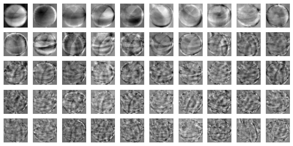
그래프 그리기
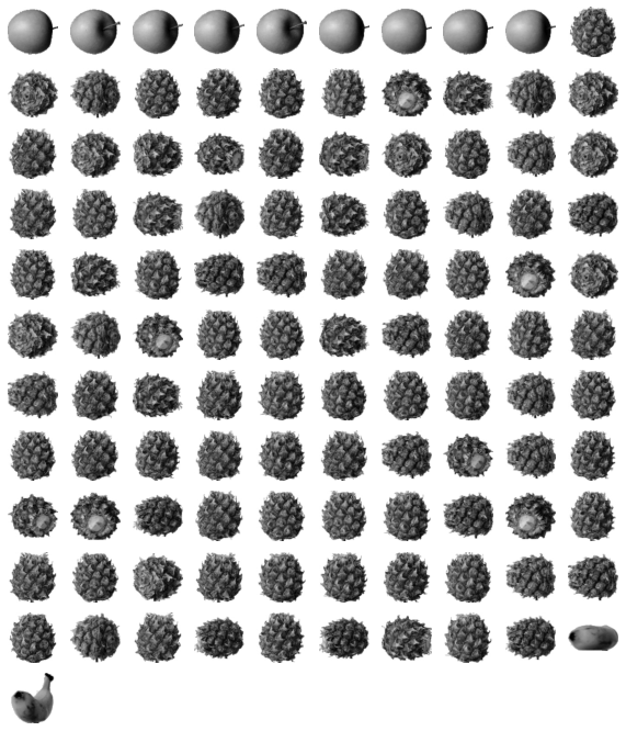
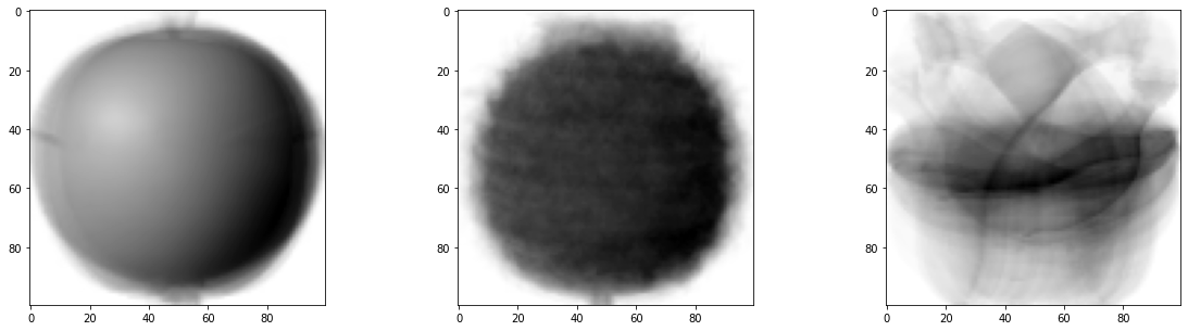
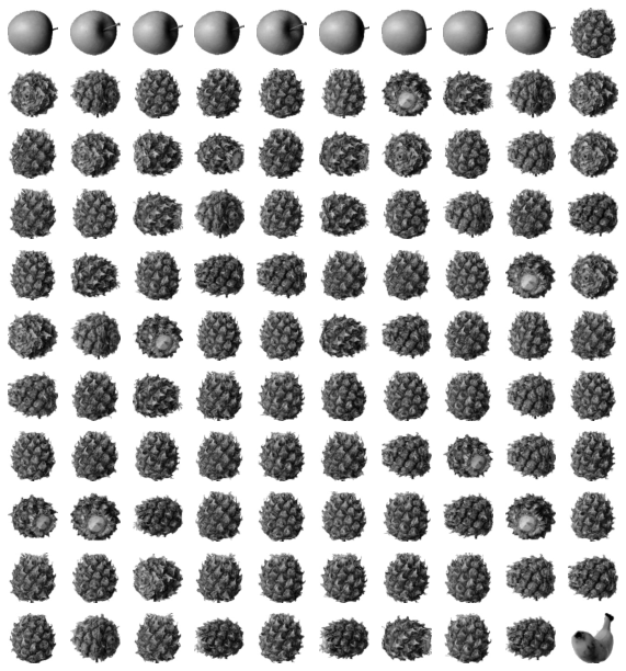
draw_fuits()함수를 사용해서 이 주성분을 그림으로 그려보자.
1 2 3 4 5 6 7 8 9 10 11 12 13 14 15 16 17 18
import matplotlib.pyplot as plt
defdraw_fruits(arr, ratio=1): n = len(arr) # n은 샘플 개수입니다 # 한 줄에 10개씩 이미지를 그립니다. 샘플 개수를 10으로 나누어 전체 행 개수를 계산합니다. rows = int(np.ceil(n/10)) # 행이 1개 이면 열 개수는 샘플 개수입니다. 그렇지 않으면 10개입니다. cols = n if rows < 2else10 fig, axs = plt.subplots(rows, cols, figsize=(cols*ratio, rows*ratio), squeeze=False) for i inrange(rows): for j inrange(cols): if i*10 + j < n: # n 개까지만 그립니다. axs[i, j].imshow(arr[i*10 + j], cmap='gray_r') axs[i, j].axis('off') plt.show()
0.9933333333333334
0.051814031600952146
/usr/local/lib/python3.7/dist-packages/sklearn/linear_model/_logistic.py:818: ConvergenceWarning: lbfgs failed to converge (status=1):
STOP: TOTAL NO. of ITERATIONS REACHED LIMIT.
Increase the number of iterations (max_iter) or scale the data as shown in:
https://scikit-learn.org/stable/modules/preprocessing.html
Please also refer to the documentation for alternative solver options:
https://scikit-learn.org/stable/modules/linear_model.html#logistic-regression
extra_warning_msg=_LOGISTIC_SOLVER_CONVERGENCE_MSG,
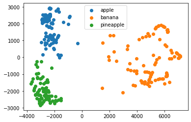
차원 축소된 데이터를 k-평균 알고리즘에 추가한다.
1 2 3 4
from sklearn.cluster import KMeans
km = KMeans(n_clusters=3, random_state=42)
km.fit(fruits_pca)
print(np.unique(km.labels_, return_counts = True))