chapter_5_1
결정 트리
- 결정 트리로 다음 문제를 해결해 보자
- 와인 캔에 인쇄된 알코올 도수, 당도, pH값으로 와인 종류를 구별해야 한다.
로지스틱 회귀로 와인 분류하기
- 우선 로지스틱 회귀로 문제 해결을 시도해본다.
데이터 불러오기
- 와인데이터
- alcohol(알고올 도수), sugar(당도), pH(산도)
- 클래스 0 = 레드 와인
- 클래스 1 = 화이트 와인
1 | import pandas as pd |
| alcohol | sugar | pH | class | |
|---|---|---|---|---|
| 0 | 9.4 | 1.9 | 3.51 | 0.0 |
| 1 | 9.8 | 2.6 | 3.20 | 0.0 |
| 2 | 9.8 | 2.3 | 3.26 | 0.0 |
| 3 | 9.8 | 1.9 | 3.16 | 0.0 |
| 4 | 9.4 | 1.9 | 3.51 | 0.0 |
  <script>
    const buttonEl =
      document.querySelector('#df-ed50d596-f5ff-4ae2-a52f-cd3b0b3d75ad button.colab-df-convert');
    buttonEl.style.display =
      google.colab.kernel.accessAllowed ? 'block' : 'none';

    async function convertToInteractive(key) {
      const element = document.querySelector('#df-ed50d596-f5ff-4ae2-a52f-cd3b0b3d75ad');
      const dataTable =
        await google.colab.kernel.invokeFunction('convertToInteractive',
                                                 [key], {});
      if (!dataTable) return;

      const docLinkHtml = 'Like what you see? Visit the ' +
        '<a target="_blank" href=https://colab.research.google.com/notebooks/data_table.ipynb>data table notebook</a>'
        + ' to learn more about interactive tables.';
      element.innerHTML = '';
      dataTable['/images/chapter_5_1/output_type'] = 'display_data';
      await google.colab./images/chapter_5_1/output.render/images/chapter_5_1/output(dataTable, element);
      const docLink = document.createElement('div');
      docLink.innerHTML = docLinkHtml;
      element.appendChild(docLink);
    }
  </script>
</div>
- info()
- 결측치 확인 / 변수 타입
1 | wine.info() |
<class 'pandas.core.frame.DataFrame'>
RangeIndex: 6497 entries, 0 to 6496
Data columns (total 4 columns):
 #   Column   Non-Null Count  Dtype
---  ------   --------------  -----
 0   alcohol  6497 non-null   float64
 1   sugar    6497 non-null   float64
 2   pH       6497 non-null   float64
 3   class    6497 non-null   float64
dtypes: float64(4)
memory usage: 203.2 KB
1 | wine.describe() |
| alcohol | sugar | pH | class | |
|---|---|---|---|---|
| count | 6497.000000 | 6497.000000 | 6497.000000 | 6497.000000 |
| mean | 10.491801 | 5.443235 | 3.218501 | 0.753886 |
| std | 1.192712 | 4.757804 | 0.160787 | 0.430779 |
| min | 8.000000 | 0.600000 | 2.720000 | 0.000000 |
| 25% | 9.500000 | 1.800000 | 3.110000 | 1.000000 |
| 50% | 10.300000 | 3.000000 | 3.210000 | 1.000000 |
| 75% | 11.300000 | 8.100000 | 3.320000 | 1.000000 |
| max | 14.900000 | 65.800000 | 4.010000 | 1.000000 |
  <script>
    const buttonEl =
      document.querySelector('#df-decc42d0-d914-4603-8cd7-d87f4c9e480a button.colab-df-convert');
    buttonEl.style.display =
      google.colab.kernel.accessAllowed ? 'block' : 'none';

    async function convertToInteractive(key) {
      const element = document.querySelector('#df-decc42d0-d914-4603-8cd7-d87f4c9e480a');
      const dataTable =
        await google.colab.kernel.invokeFunction('convertToInteractive',
                                                 [key], {});
      if (!dataTable) return;

      const docLinkHtml = 'Like what you see? Visit the ' +
        '<a target="_blank" href=https://colab.research.google.com/notebooks/data_table.ipynb>data table notebook</a>'
        + ' to learn more about interactive tables.';
      element.innerHTML = '';
      dataTable['/images/chapter_5_1/output_type'] = 'display_data';
      await google.colab./images/chapter_5_1/output.render/images/chapter_5_1/output(dataTable, element);
      const docLink = document.createElement('div');
      docLink.innerHTML = docLinkHtml;
      element.appendChild(docLink);
    }
  </script>
</div>
표준화 작업
- 배열로 바꿔서 진행
1 | data = wine[['alcohol', 'sugar', 'pH']].to_numpy() # 참고할 데이터 |
훈련데이터와 테스트데이터로 분리
- train_test_split() 함수는 설정값을 지정하지 않으면 25%를 테스트 세트로 지정한다.
- 이번엔 샘플 개수가 충분히 많으므로 20% 정도만 테스트 세트로 나눈다.
- test = 0.2 에는 이러한 의도가 담겨 있다.
1 | from sklearn.model_selection import train_test_split |
(5197, 3) (1300, 3)
- 이제 표준화 진행하자
1 | from sklearn.preprocessing import StandardScaler |
모델 만들기
로지스틱 회귀
- 표준변환된 train_scaled와 test_scaled를 사용해 로지스틱 회귀 모델을 훈련한다.
1 | from sklearn.linear_model import LogisticRegression |
0.7808350971714451
0.7776923076923077
[[ 0.51270274  1.6733911  -0.68767781]] [1.81777902]
- 점수가 높게 나오지 않았다.
- 결정 트리를 이용하여 좀 더 쉽게 문제를 해결해보자
로지스틱 회귀
- 수식
의사결정트리의 기본 알고리즘을 활용해서, MS, 구글 등 이런 회사들이 신규 알고리즘을 만듬
- XGBoost, lightGBM, CatBoost
- 캐글 정형데이터
- lightGBM (지금 현재 실무에서 많이 쓰임)
- 4월 말까지는 코드에 집중. 대회 나감
- PPT (알고리즘 소개)
결정 트리 (Decision Tree)
- 스무 고개와 같다.
- 질문을 하나씩 던져서 정답과 맞춰가는 것이다.
- 표준화된 훈련 세트를 이용하여 결정트리를 사용해 본다.
1 | from sklearn.tree import DecisionTreeClassifier |
0.996921300750433
0.8592307692307692
- 위 코드의 두 결과는 차이가 있다.
- 두 결과가 유사하게 나와야 한다.
- 앞으로 ‘가지치기’에서 차이를 좁히는 과정을 진행한다.
1 | # 현재 트리의 형태를 출력해본다. |
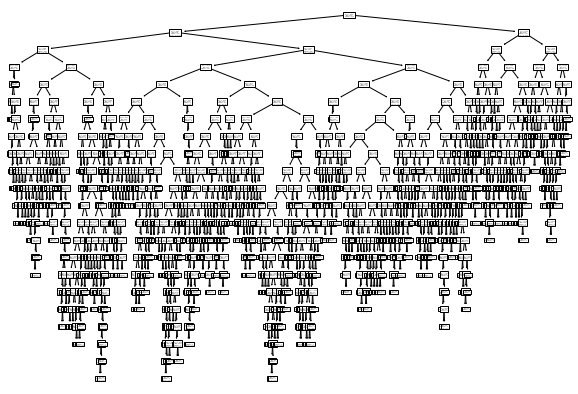
- 과대적합이 나오는 이유 : 조건식을 걸기 때문
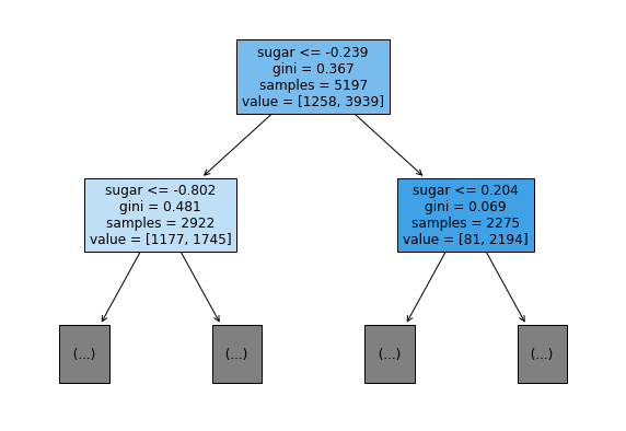
1 | # plot_tree()함수에서 트리의 깊이를 제한하여 출력해 본다. |
- 불순도 : 운동회 ox 퀴즈에서 정답을 맞힌 사람만 살아남는 것과 같은 원리
가지치기
- 과대적합을 방지하기 위한 것
- 가지치기를 통해 두 결과가 유사하게 출력된다.
1 | dt = DecisionTreeClassifier(max_depth = 3, random_state=42) # max_depth 매개변수 조절을 통해 가지치기 한다. |
0.8454877814123533
0.8415384615384616
- 훈련 세트와 테스트 성능이 유사하게 출력되었다.
- 이런 모델을 트리 그래프로 그린다면 훨씬 이해햐기 쉬울 것이다.
1 | plt.figure(figsize=(20,15)) |
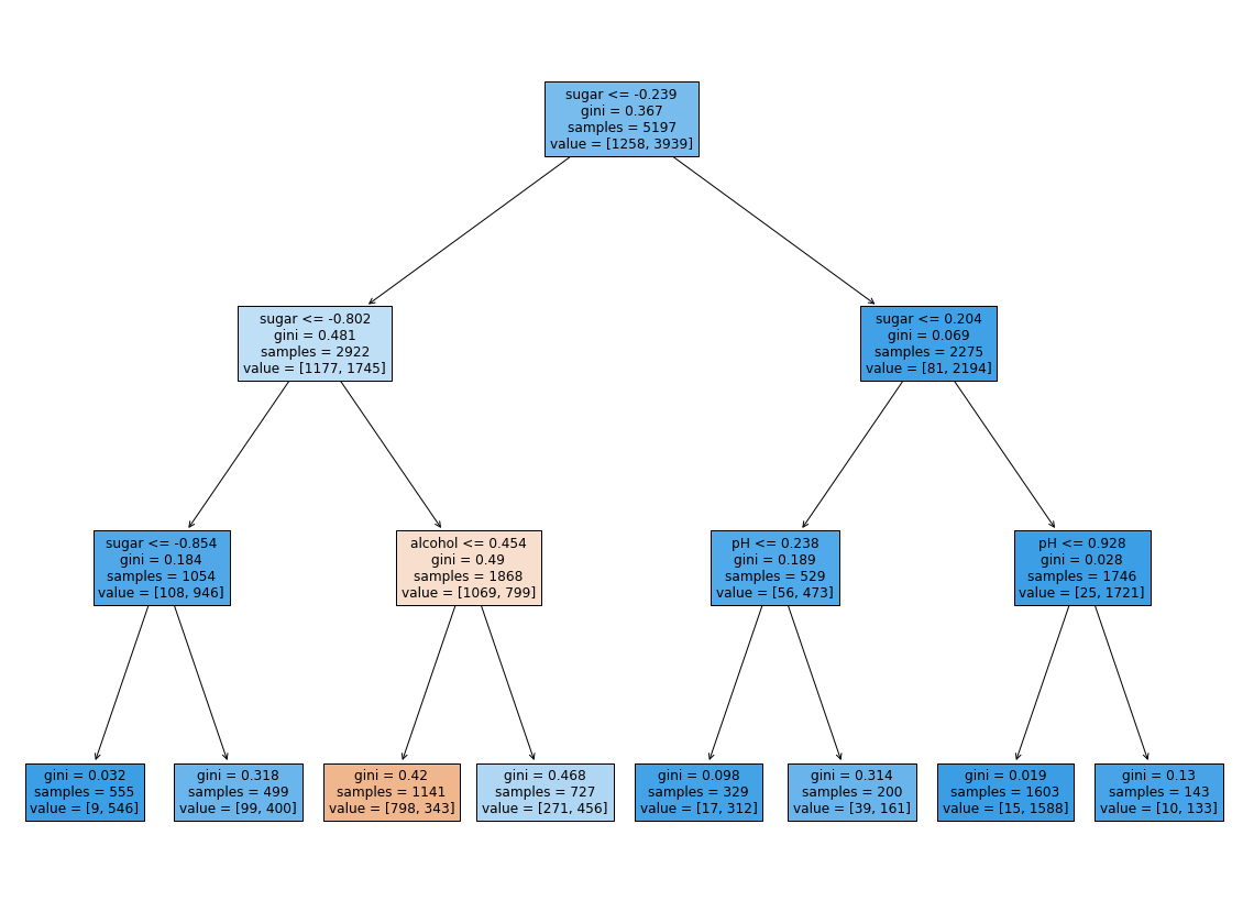
훨씬 보기 좋게 출력되었다.
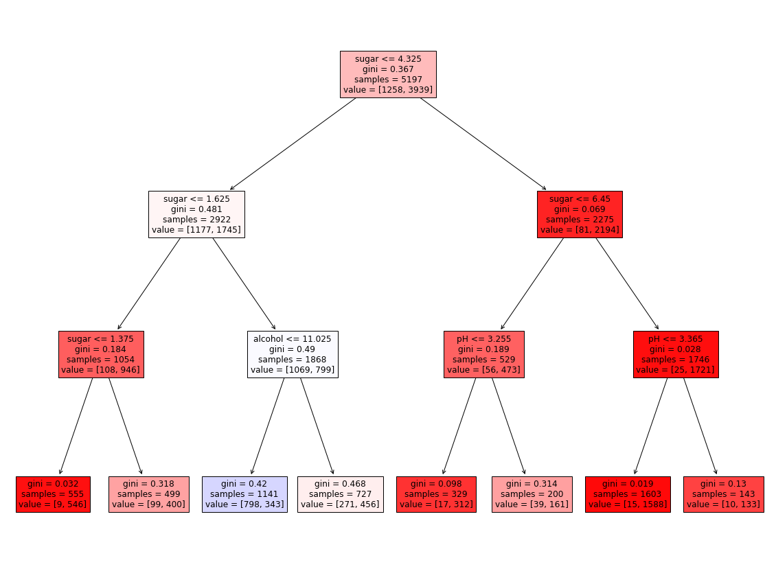
루트 노트
- 당도(sugar)를 기준으로 훈련세트를 나눈다.
깊이 1의 노드
- 모두 당도(sugar)를 기준으로 훈련 세트를 나눈다.
깊이 2의 노드
- 맨 왼쪽의 노드만 당도를 기준으로 나눈다.
- 왼쪽에서 두 번째 노드는 알고올 도수(alcohol)를 기준으로 나눈다.
- 오른쪽 두 노드는 pH를 기준으로 나눈다.
리프 노드
- 왼쪽에서 3번째에 있는 노드만 음성 클래스가 더 많다.
- 이 노드에 도착해야만 레드 와인으로 예측한다.
- 이 노드에 도달하려면 -0.802 < sugar < -0.239, alcohol < -0.454 라는 조건을 만족해야 한다.
- 즉, -0.802 < sugar < -0.239, alcohol < -0.454 이면 레드와인이다
- 왼쪽에서 3번째에 있는 노드만 음성 클래스가 더 많다.
그런데 -0.802라는 음수로 된 당도를 어떻게 설명해야할까?
- 좀 더 설명하기 쉽게 바꿔보자.
특성값의 스케일은 결정 트리 알고리즘에 아무런 영향을 미치지 않는다.
따라서 표준화 전처리를 할 필요가 없다.
전처리하기 전의 훈련 세트(train_input)와 테스트 세트(test_input)로 결정 트리 모델을 다시 훈련해 본다.
1 | dt = DecisionTreeClassifier(max_depth=3, random_state=42) |
0.8454877814123533
0.8454877814123533
- 정확히 같은 결과가 나왔다.
- 트리도 그려보자.
1 | plt.figure(figsize=(20, 15)) |
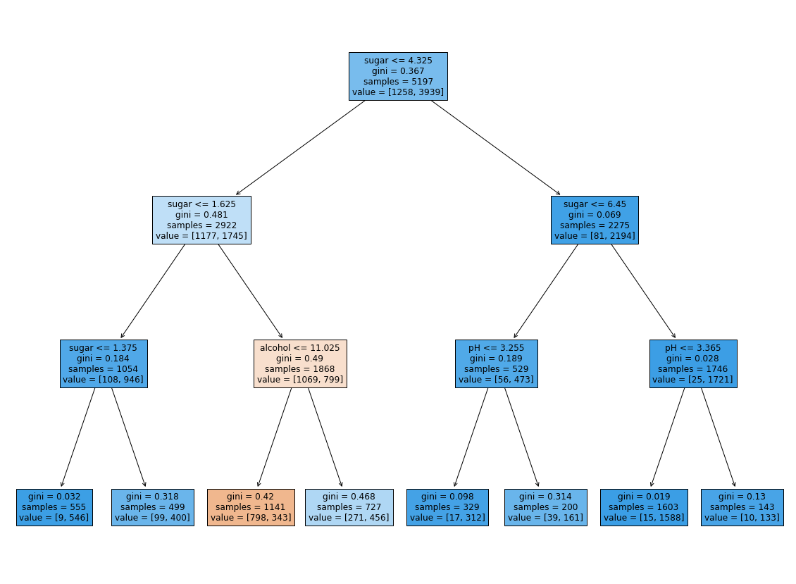
같은 트리지만 특성값을 표준점수로 바꾸지 않았기에 이해하기 훨씬 쉽다.
- 적어도 당도를 음수로 표기하는 것보단 보기 좋다.
다음 조건을 만족하는 것이 레드 와인이다.
- (1.625 < sugar < 4.325) AND (alcohol < 11.025) = 레드 와인
특성 중요도
- 결정 트리는 어떤 특성이 가장 유용한지 나타내는 특성 중요도를 계산해준다.
- 이 트리의 루트 노드와 깊이 1에서 sugar를 사용했기 때문에 아마 sugar가 가장 유용한 특성 중 하나일 것이다.
- 특성 중요도는 결정 트리 모델의 feature_importances_ 속성에 저장되어 있다.
1 | print(dt.feature_importances_) |
[0.12345626 0.86862934 0.0079144 ]
alcohol ,sugar, ph 순서이기 때문에 두 번째인 sugar의 중요도가 가장 높은 것을 알 수 있다.
번외
1 | import graphviz |
'decision_tree_graphivz.png'
1 | from matplotlib.colors import ListedColormap, to_rgb |
- Reference : 혼자 공부하는 머신러닝 + 딥러닝
You need to set
install_url to use ShareThis. Please set it in _config.yml.Like this article? Support the author with
Afdian.netAlipay Buy me a coffeePatreon
You forgot to set the
Wechatbusiness or currency_code for Paypal. Please set it in _config.yml.Comments
You forgot to set the
shortname for Disqus. Please set it in _config.yml.